Welcome to the CWE CVE Benchmark¶

This is the community collaboration site to build a CVE-CWE mapping benchmark and leaderboard.

Slide from Call for Community Collaboration from Vulnerability Root Cause Mapping with CWE: Challenges, Solutions, and Insights from Grounded LLM-based Analysis

Introduction ↵

Introduction¶

About this

This section outlines the Why, What, When, How for the CWE Root Cause Mapping Benchmark and Leaderboard Community Collaboration Group.

Why¶

Background¶

Accurate CVE-CWE Root Cause Mapping (RCM) facilitates trend analysis, investment prioritization, exploitability insights, and SDLC feedback.

Per Vulnerability Root Cause Mapping with CWE: Challenges, Solutions, and Insights from Grounded LLM-based Analysis, the Value of RCM is that it:

Enables vulnerability trend analysis and greater visibility into their patterns over time
Illuminates where investments, policy, and practices can address the weaknesses responsible for product vulnerabilities so that they can be eliminated
Provides further insight to potential “exploitability” based on weakness type
Provides valuable feedback loop into an SDLC or architecture design planning

But there are known mapping quality issues.

Purpose¶

To address CVE-CWE Root Cause Mapping Quality issues by enabling a Benchmark dataset and Leaderboard that allows sharing of common measurements and improvement of tools/technology.

Advancing CWE mapping technology, showcasing technology and talent via a leaderboard based on the benchmark, and ultimately improving CVE-CWE data quality for us all!

Vision¶

The CVE CWE Root Cause Mapping Benchmark

allows measurement and improvement of tools/processes to address the CVE-CWE Quality issues: from ChatBots to Bulk assignment/validation.
is used by industry and academia
is endorsed by MITRE CWE as being fit for purpose
has an associated Leaderboard where people showcase their tools and talent against the CVE CWE Root Cause Mapping Benchmark
promotes doing the right thing e.g. using the Reference content, and additional CVE info to do CWE mapping
reflects real world usage and CWE assignment by CWE experts (MITRE CWE Top 25). This includes the Root Cause CWE and other CWEs for a given CVE.

What and When¶

Deliverables Q1 2026¶

a presentation submittal for FIRST VulnCon 2026 (Scottsdale, AZ is the venue)
a paper
a published known-good CWE-RCM dataset that can be used by industry and academia to improve CWE RCM.
a published leaderboard where people can compete using the benchmark with results from at least 3 tools.

How¶

Resources We Have¶

Access to the non-public MITRE CWE Top25 2023, 2022 datasets + guidance/expertise of the MITRE CWE team + participation in the MITRE CWE RCMWG.
Top SME participants: Data scientists, architects, developers, academics, CNAs, MITRE CWE.
Access to community

Components¶


flowchart TD
    A[Benchmark Dataset] -->|Gold reference| C[Comparison Tool]
    B[Assignment Tool] -->|Outputs CWE assignments| H
    D[Tool Guidance] -->|Guides implementation of| B
    E[Comparison Requirements] -->|Guides implementation of| C
    C 
    G[Benchmark Dataset Guidance] -->|Guides implementation of| A[Benchmark Dataset]
    H[Assigned CWE Dataset] -->|Dataset to evaluate| C[Evaluation Tool]
    J[Scoring Algorithms] -->|Scoring Logic| C[Evaluation Tool]


    C[Evaluation Tool] --> |Outputs| I[Evaluation Results]
    I[Evaluation Results]-->|Ranked on| F[Leaderboard]


    classDef document fill:#f9f,stroke:#333,stroke-width:2px;
    classDef tool fill:#bbf,stroke:#333,stroke-width:2px;
    classDef data fill:#bfb,stroke:#333,stroke-width:2px;

    class E,D,G document;
    class B,C,F tool;
    class A,H,I data;

    click G "../../requirements/dataset" "View Dataset Requirements"
    click E "../../requirements/comparison" "View Dataset Requirements"
    click D "../../requirements/tool_guidance" "View Dataset Requirements"
    click J "../../scoring/overview/#scoring-approaches" "Scoring Approaches"

Exploratory Data Analysis¶

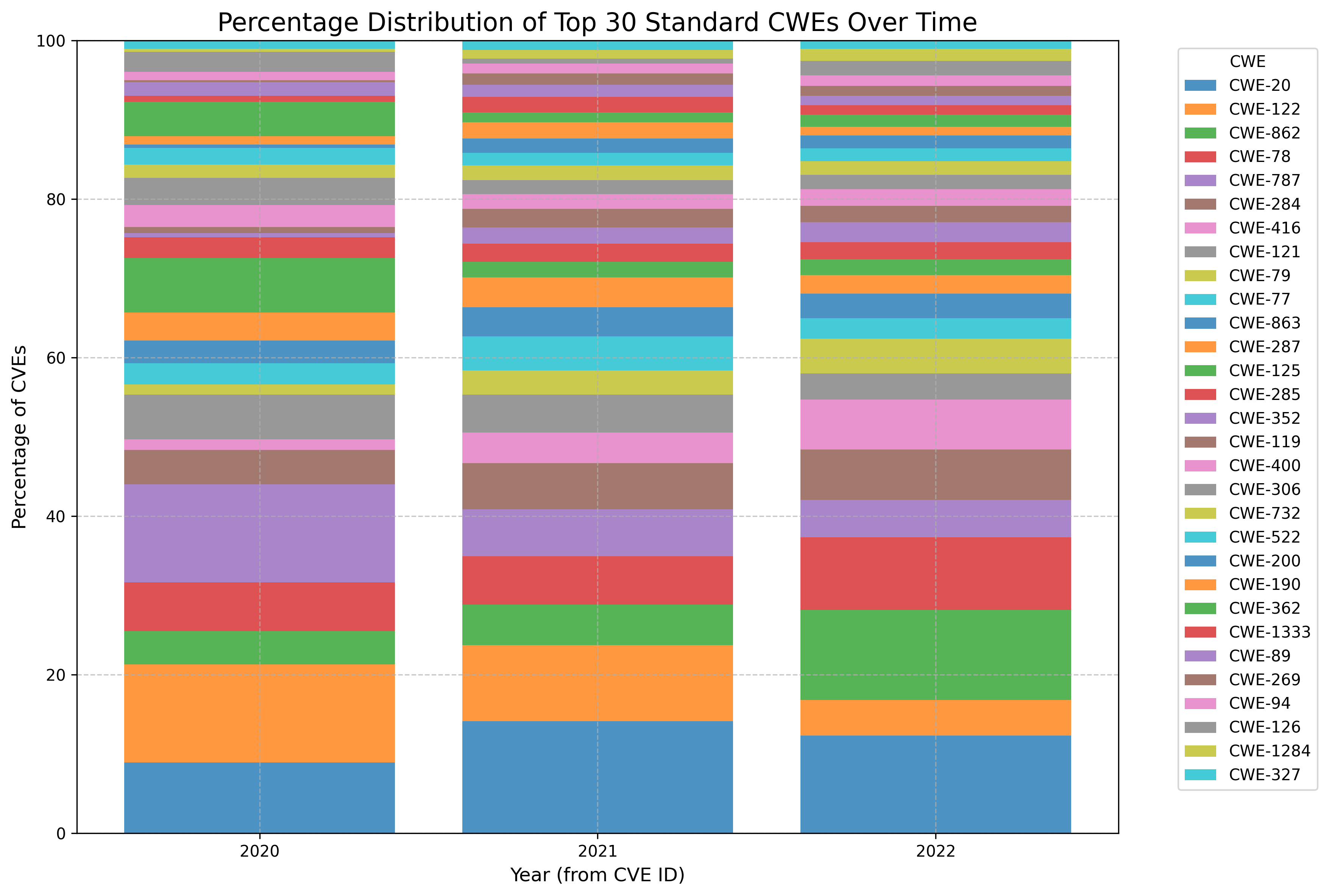
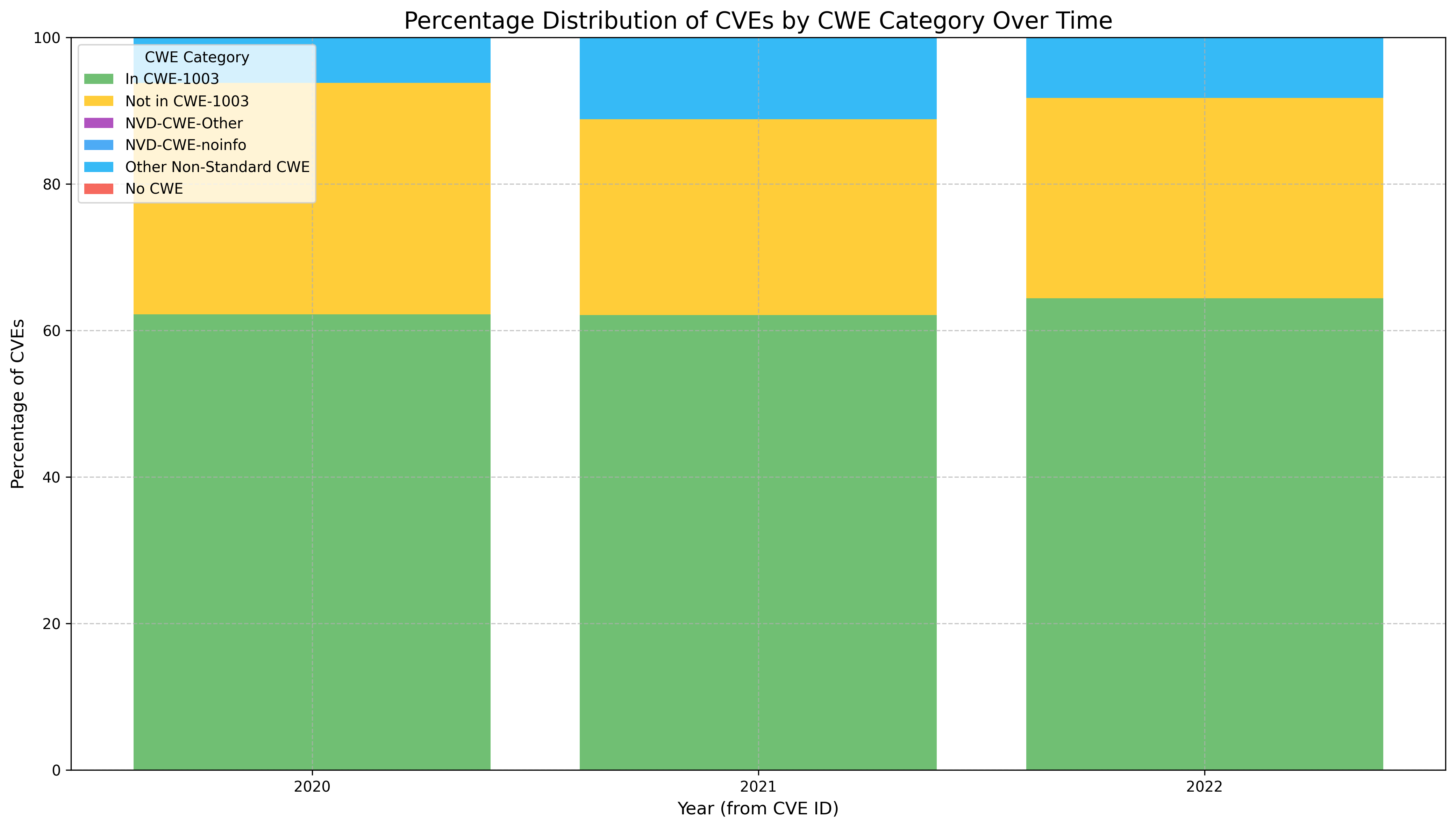
See Top25 dataset EDA.

See CWE Counts of all published CVEs.

Benchmark Dataset¶

See dataset requirements that defines characteristics that address Limitations of existing RCM datasets.

Benchmark Comparison Algorithm¶

See comparison requirements.

See scoring algorithms

Guidance on Implementing Tools¶

See tool guidance.

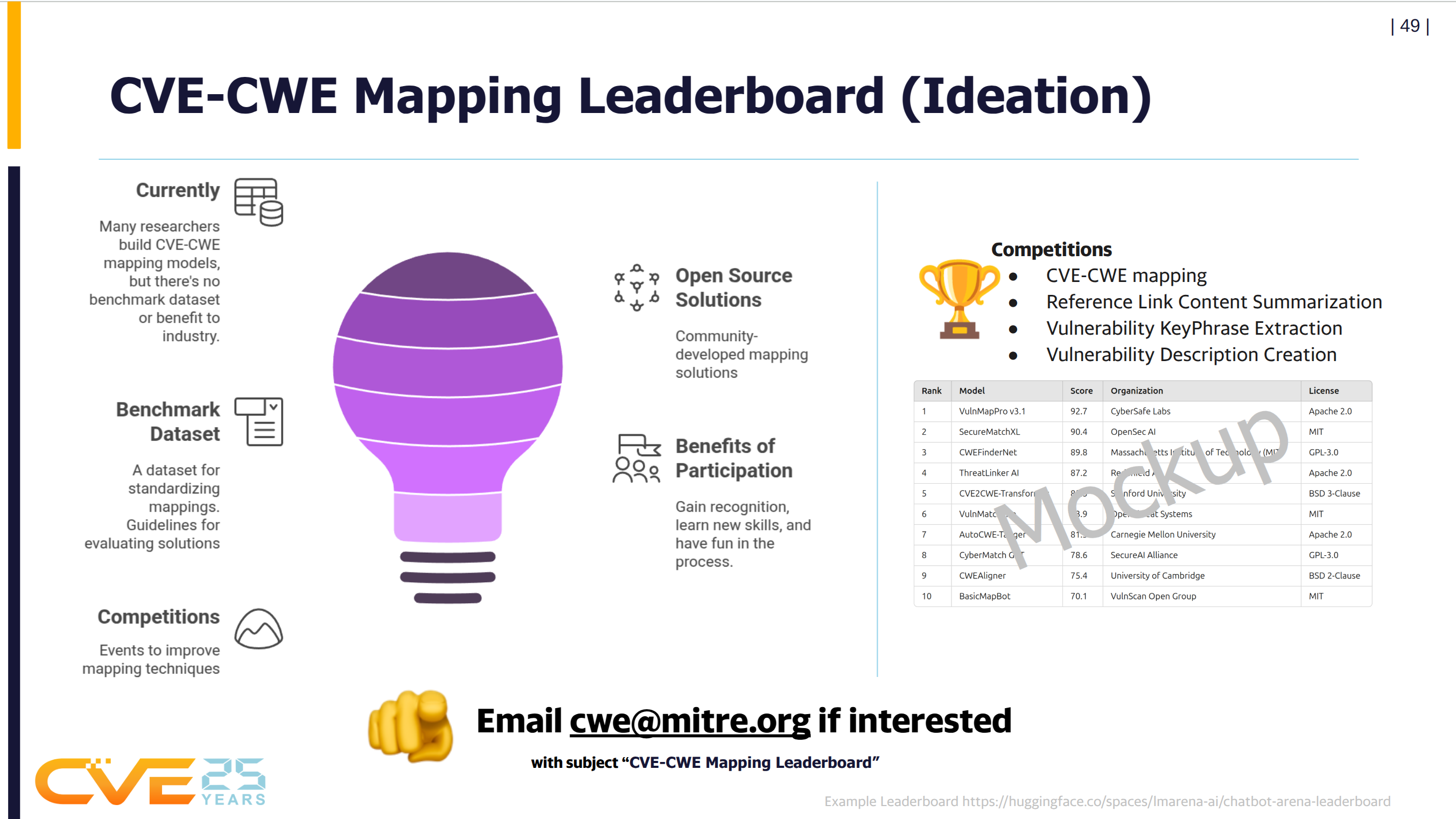
Leaderboard¶

Hosting e.g. HuggingFace
Battle format and algorithm e.g. https://huggingface.co/spaces/lmarena-ai/chatbot-arena-leaderboard
UX
Requirements to participate e.g. OSS License

Ended: Introduction

Requirements ↵

CVE-CWE Root Cause Mapping Dataset Requirements¶

Overview

This section outlines the requirements for creating a comprehensive benchmark dataset for CVE-CWE Root Cause mapping.

Table of Contents¶

CVE-CWE Root Cause Mapping Dataset Requirements
Table of Contents
Coverage Requirements
Quality Requirements
Data Sources
- Datasets
- CVE Info
Validation
References
ToDo

Coverage Requirements¶

REQ_COVERAGE_PRACTICAL_CWES: The dataset MUST include all CWEs used in practice i.e. a CWE is used in at least 1 published CVE(s) (approximately 400-500).

REQ_COVERAGE_CWE1003_VIEW: The dataset MUST include all CWEs in CWE-1003 view (approximately 130).

REQ_COVERAGE_TOP25_CWES: The dataset MUST include all CWEs in https://cwe.mitre.org/top25/ from 2019 to current 2024 CWE Top 25.

See https://github.com/CWE-CVE-Benchmark/CWE_analysis/blob/main/data_in/Top25_per_year.tsv that lists these Top25 per year.

REQ_COVERAGE_ALL_CWES: The dataset MAY include all CWEs (approximately 1000).

REQ_COVERAGE_RECENT_CVES: The dataset SHOULD include mostly CVEs from recent CVE publication years to reflect current reality. The dataset should be expanded in reverse chronological order until sufficient examples are collected for each targeted CWE class.

REQ_COVERAGE_MIN_ENTRIES_PER_CWE: The dataset MUST include at least 5 entries per CWE (if such CVE examples exist).

REQ_COVERAGE_DIVERSE_DESCRIPTIONS: For a given CWE, the dataset MUST include CVE Descriptions that are sufficiently different per CVE Description, measured quantitatively using fuzzy and semantic similarity against a threshold.

REQ_COVERAGE_MULTIPLE_CWES: The dataset MUST include CVEs with multiple CWEs assigned, as reflected by the Top25 datasets.

REQ_COVERAGE_REF_CONTENT_RAW: The dataset MUST include CVE Reference Link Content as the raw content in text format.

REQ_COVERAGE_REF_CONTENT_SUMMARY: The dataset MUST include CVE Reference Link Content as a summary (e.g., as in https://github.com/CyberSecAI/cve_info_refs).

REQ_COVERAGE_LICENSE: The dataset MUST include a LICENSE as agreed by MITRE CWE.

REQ_COVERAGE_README: The dataset MUST include a README.

REQ_COVERAGE_MAINTENANCE_PLAN: The dataset MUST include a documented Maintenance Plan.

REQ_COVERAGE_CHANGE_TRACKING: The dataset MUST include change tracking and full history (e.g., via GitHub).

REQ_COVERAGE_VALIDATION_PROCESS: The dataset MUST include a documented validation process/script that automatically validates the dataset meets the requirements.

REQ_COVERAGE_FEEDBACK_PROCESS: The dataset MUST include a documented feedback process.

REQ_COVERAGE_SEMVER: The dataset MUST use Semantic Versioning.

REQ_COVERAGE_KEYPHRASES: The dataset SHOULD include the CVE Description Vulnerability KeyPhrases (e.g., as in https://github.com/CyberSecAI/cve_info).

REQ_COVERAGE_NO_REJECTED_CVES: The dataset SHOULD NOT include CVEs that are Rejected at the time of creating the dataset. Over time, CVEs in the dataset may become REJECTED, and these should be removed or identified/labeled.

REQ_COVERAGE_NO_DEPRECATED_CWES: The dataset SHOULD NOT include CWEs that are Deprecated, Obsolete, or Prohibited at the time of creating the dataset. Over time, CWEs in the dataset may become deprecated or obsolete, and these should be removed or identified/labeled.

REQ_COVERAGE_TOOL_AGNOSTIC: The dataset MUST be tool/solution agnostic. E.g. it MUST NOT include prompts per https://huggingface.co/datasets/AI4Sec/cti-bench/viewer/cti-rcm?views%5B%5D=cti_rcm&row=1

REQ_CONSENSUS_CNA_SCORE: The dataset SHOULD include a consensus score that reflects the level of agreement between CNAs in assigning CWEs to a CVE (e.g., if Red Hat, Microsoft, and IBM all select the same CWE ID for a specific CVE, then the score is 100).

REQ_CONSENSUS_DESC_SCORE: The dataset SHOULD include a consensus score that reflects the level of agreement between CWEs assigned for similar CVE descriptions. See https://github.com/CyberSecAI/cve_dedup/.

Quality Requirements¶

REQ_QUALITY_KNOWN_GOOD: The dataset MUST be known-good (i.e., the assigned CWE(s) is correct). Observed examples provide high-quality mappings but should be limited to those published after 2015 to ensure consistency with modern CVE description standards.

REQ_QUALITY_UTF8: The dataset MUST be UTF-8 only.

REQ_QUALITY_SCHEMA_VALIDATOR: The dataset MUST have a schema and validator script that is part of the dataset.

REQ_QUALITY_LOW_QUALITY_CVES: The dataset MUST include and identify low-quality CVEs. A sufficient number of low-info CVEs are labeled such that the results for those CVEs can be isolated to e.g., test for hallucinations/grounding.

REQ_QUALITY_DATA_SPLITS: The dataset MUST have train/validate/test splits.

REQ_QUALITY_PRESERVE_ISSUES: The dataset SHOULD NOT fix existing typos or other issues in the CVEs.

REQ_QUALITY_ABSTRACTION_CHECK: The dataset MUST check abstraction levels of CWEs and verify that high-level CWEs (such as Pillars) are only included where no lower-level CWE exists.

Data Sources¶

Datasets¶

REQ_DATASRC_TOP25_2023: The dataset SHOULD use Top25 2023 (approximately 7K entries) as a source.

REQ_DATASRC_TOP25_2022: The dataset SHOULD use Top25 2022 (approximately 7K entries) as a source.

REQ_DATASRC_NO_OBSERVED_EXAMPLES: The dataset SHOULD NOT use CWE Observed Examples published before 2015, as many are worded differently from modern CVE descriptions. Observed examples from 2015 onwards may be included as they provide high-quality mappings.

CVE Info¶

REQ_CVEINFO_JSON_5_0: https://github.com/CVEProject/cvelistV5 is the canonical source for CVE descriptions & references.

Validation¶

REQ_VALIDATION_SCHEMA: JSON schema validation must pass with schema.json.

REQ_VALIDATION_REQUIREMENTS: The dataset must be validated against the requirements.

REQ_VALIDATION_STATISTICS: Basic statistics (token lengths, keyphrase counts) must be generated.

REQ_VALIDATION_CONSENSUS_SCORES: Consensus scores for both CNA agreement and similar CVE descriptions must be calculated and validated.

References¶

RFC 2119 for definitions of "SHOULD", "MUST", etc.
CWE-1003 View for maintaining consistency in CWE assignments
CWE Top 25 for priority CWE coverage
Developer View (View-699) for comprehensive coverage approach

ToDo¶

Define Known-Good. Specify the validation standard and process.
Define Quantitative Metrics: Specify thresholds/methods for sufficiently different
Define Qualitative Labels: Specify criteria for low-quality
Specify methodology for calculating consensus scores (both CNA and description-based)
Define minimum consensus score thresholds for creating high-quality benchmark subsets

CVE-CWE Benchmark Comparison Algorithm Requirements¶

Overview

This section outlines the requirements for the algorithm that evaluates automated CWE assignments against the gold-standard benchmark dataset.

Table of Contents¶

CVE-CWE Benchmark Comparison Algorithm Requirements
Table of Contents
Algorithm Core Requirements
CWE Matching Requirements
Multiple CWE Handling Requirements
Abstraction Level Requirements
Evaluation Metrics Requirements
Grounding and Low-Information Requirements
Implementation Requirements
References

Algorithm Core Requirements¶

REQ_ALGO_MULTI_LABEL: The comparison algorithm MUST treat CWE assignment as a multi-label classification problem.

REQ_ALGO_HIERARCHICAL: The comparison algorithm MUST incorporate the hierarchical nature of CWEs in its matching logic.

REQ_ALGO_PARTIAL_CREDIT: The comparison algorithm MUST support partial credit for related but non-exact CWE matches.

REQ_ALGO_EXPLAINABLE: The comparison algorithm MUST provide explanations for why specific matches were scored in a particular way.

CWE Matching Requirements¶

REQ_MATCH_EXACT: The algorithm MUST identify and give full credit (score = 1.0) for exact CWE ID matches.

REQ_MATCH_UNRELATED: The algorithm MUST identify unrelated CWEs (different branches with no close common ancestor) and give no credit (score = 0).

REQ_MATCH_CUSTOMIZABLE: The algorithm MUST allow customizable weights for each degree of match to compute similarity scores.

REQ_MATCH_CWE_GRAPH: The algorithm MUST use the official CWE 1000 View graph to determine relationships between CWEs.

Multiple CWE Handling Requirements¶

REQ_MULTI_LABEL_BASED: The algorithm MUST support multi-label-based metrics for evaluating individual CWE predictions across all CVEs.

Abstraction Level Requirements¶

REQ_ABSTRACT_TRACKING: The algorithm MUST track the abstraction level (Pillar, Class, Base, Variant) of each CWE.

REQ_ABSTRACT_FILTERING: The algorithm MUST support filtering or grouping results by abstraction level.

REQ_ABSTRACT_SEPARATE_METRICS: The algorithm MUST calculate metrics separately for different abstraction levels when requested.

REQ_ABSTRACT_MISMATCH: The algorithm MUST identify and report when predictions match at a different abstraction level than the gold standard.

REQ_ABSTRACT_PREFERENCE: The algorithm SHOULD implement a preference for Base/Variant level matches over Class/Pillar matches, in accordance with CWE mapping guidance.

Evaluation Metrics Requirements¶

REQ_METRIC_EXACT_MATCH: The algorithm MUST calculate and report the Exact Match Rate (EMR) - the proportion of CVEs where predicted CWE sets exactly match gold CWE sets.

REQ_METRIC_AT_LEAST_ONE: The algorithm MUST calculate and report the At Least One Match Rate - the proportion of CVEs where at least one gold CWE was correctly predicted.

REQ_METRIC_PRECISION: The algorithm MUST calculate and report Precision (Positive Predictive Value) based on true and false positives.

REQ_METRIC_RECALL: The algorithm MUST calculate and report Recall (Sensitivity) based on true positives and false negatives.

REQ_METRIC_F1: The algorithm MUST calculate and report the F1 Score as the harmonic mean of precision and recall.

REQ_METRIC_BALANCED_ACCURACY: The algorithm MUST calculate and report Balanced Accuracy, accounting for class imbalance by averaging recall across CWE classes.

REQ_METRIC_SOFT_VERSIONS: The algorithm MUST support "soft" versions of precision, recall, and F1 that incorporate partial match scores.

REQ_METRIC_BREAKDOWN: The algorithm SHOULD provide breakdowns of metrics by CWE frequency, abstraction level, or other relevant criteria.

REQ_METRIC_MACRO_MICRO: The algorithm SHOULD calculate both micro and macro averages for precision, recall, and F1 when appropriate.

REQ_METRIC_CONFIDENCE: The algorithm SHOULD incorporate confidence intervals or uncertainty measures for the reported metrics when sample sizes permit.

Grounding and Low-Information Requirements¶

REQ_GROUND_HALLUCINATION: The algorithm MUST implement detection for "hallucinated" CWE assignments that have no apparent support in the CVE description.

REQ_GROUND_KEYWORD: The algorithm SHOULD use keyword/term matching to check if a CWE's characteristic terms appear in the CVE description.

REQ_GROUND_SEMANTIC: The algorithm SHOULD use semantic similarity techniques to assess if predictions are related to the CVE text content.

REQ_GROUND_SEPARATE_METRICS: The algorithm MUST report the percentage of predictions flagged as potential hallucinations.

REQ_LOW_INFO_EXCLUDE: The algorithm MUST support excluding low-information CVEs from primary evaluation metrics.

REQ_LOW_INFO_SEPARATE: The algorithm MUST report metrics with and without low-information CVEs to show their impact on overall performance.

Implementation Requirements¶

REQ_IMPL_PERFORMANCE: The algorithm MUST be efficient enough to process large CVE datasets (tens of thousands of entries) in a reasonable time.

REQ_IMPL_OUTPUT_FORMAT: The algorithm MUST produce structured output in a machine-readable format (e.g., JSON) with clear organization of metrics and results.

REQ_IMPL_DETAILED_RESULTS: The algorithm MUST provide detailed per-CVE results showing matches, scores, and classification decisions.

REQ_IMPL_SUMMARY_STATS: The algorithm MUST generate summary statistics and aggregate metrics for the entire evaluation.

REQ_IMPL_VERSION_INFO: The algorithm output report MUST include version information of: 1) the benchmark dataset used, 2) the comparison algorithm version, and 3) a timestamp indicating when the comparison was run.

REQ_IMPL_LOGGING: The algorithm MUST produce a detailed log file capturing the execution process, including configuration settings used, processing steps, any warnings or errors encountered, and summary of results. This log file MUST be separate from the main output report and should provide sufficient information for debugging and audit purposes.

REQ_IMPL_VISUALIZATION: The algorithm SHOULD generate visualizations of results such as confusion matrices, precision-recall curves, or match distributions.

REQ_IMPL_DOCUMENTABILITY: The algorithm MUST be well-documented, with clear explanations of all metrics, weighting schemes, and decision processes.

REQ_IMPL_REPRODUCIBILITY: The algorithm MUST produce reproducible results given the same input data and configuration parameters.

REQ_IMPL_EXTENSIBILITY: The algorithm SHOULD be designed to be extensible for future CWE versions, additional metrics, or enhanced matching techniques.

REQ_IMPL_SEMVER: The algorithm implementation and its scripts MUST use Semantic Versioning to clearly indicate compatibility and feature changes between releases.

References¶

CWE - CVE → CWE Mapping "Root Cause Mapping" Guidance
RFC 2119 for definitions of "SHOULD", "MUST", etc.
QualiTagger: Automating software quality detection in issue trackers
balanced_accuracy_score — scikit-learn 1.6.1 documentation

Guidance on CWE Assignment Tools¶

Overview

This section provides guidance for developers creating tools that assign Common Weakness Enumeration (CWE) identifiers to Common Vulnerabilities and Exposures (CVEs).

Tools following these guidelines will produce outputs compatible with the benchmark comparison framework.

Observability and Logging¶

GUIDE_LOG_DETAILED: Tools SHOULD generate detailed log files that capture the entire CWE assignment process, including initialization, data loading, processing steps, and result generation.

GUIDE_LOG_LEVELS: Tools SHOULD implement multiple logging levels (e.g., DEBUG, INFO, WARNING, ERROR) to allow users to control the verbosity of logs.

GUIDE_LOG_FORMAT: Log entries SHOULD include timestamps, component identifiers, and hierarchical context to facilitate tracing through the assignment process.

GUIDE_LOG_ERRORS: Tools MUST log all errors and exceptions with sufficient context to understand what failed, why it failed, and the impact on results.

GUIDE_LOG_PERFORMANCE: Tools SHOULD log performance metrics such as processing time per CVE and memory usage to help identify bottlenecks.

GUIDE_LOG_CONFIG: Tools MUST log all configuration settings and parameters used for the CWE assignment run to ensure reproducibility.

Confidence Scoring¶

GUIDE_CONF_PER_CWE: Tools MUST provide a confidence score (between 0.0 and 1.0) for each CWE assigned to a CVE, indicating the tool's certainty in that specific assignment.

GUIDE_CONF_OVERALL: Tools MUST provide an overall confidence score for the complete set of CWE assignments for each CVE, which may reflect factors beyond individual CWE confidence scores.

GUIDE_CONF_THRESHOLD: Tools SHOULD allow configurable confidence thresholds below which CWEs are either flagged as uncertain or excluded from results.

GUIDE_CONF_FACTORS: Tools SHOULD document the factors considered in confidence calculations, such as information completeness, ambiguity, semantic match strength, or historical pattern data.

GUIDE_CONF_LOW_INFO: Tools MUST assign lower confidence scores when processing CVEs with minimal or vague information to indicate higher uncertainty.

Rationale and Evidence¶

GUIDE_RAT_EXPLANATION: Tools MUST provide a textual explanation for each assigned CWE, describing why that weakness type was selected for the CVE.

GUIDE_RAT_EVIDENCE: Tools MUST cite specific evidence from the CVE description or reference materials that supports each CWE assignment.

GUIDE_RAT_KEYWORDS: Tools SHOULD highlight key terms, phrases, or patterns in the CVE content that influenced the CWE selection.

GUIDE_RAT_ALTERNATIVES: Tools SHOULD identify alternative CWEs that were considered but rejected, and explain the reasoning for not selecting them.

GUIDE_RAT_HIERARCHY: When assigning a CWE, tools SHOULD explain its position in the CWE hierarchy and why that abstraction level was chosen over parent or child weaknesses.

GUIDE_RAT_REFERENCES: Tools SHOULD reference similar historical CVEs with known CWE assignments that informed the current assignment when applicable.

CWE Selection Principles¶

GUIDE_SEL_ROOT_CAUSE: Tools MUST focus on identifying the root cause weakness rather than the vulnerability impact, following CWE mapping guidance.

GUIDE_SEL_ABSTRACTION: Tools SHOULD prioritize Base and Variant level CWEs over Class level when sufficient information is available, in accordance with CWE mapping best practices.

GUIDE_SEL_MULTIPLE: Tools MUST assign multiple CWEs when a CVE exhibits multiple distinct weaknesses, rather than forcing a single classification.

GUIDE_SEL_SPECIFICITY: Tools SHOULD select the most specific applicable CWE rather than an overly general one, given sufficient evidence.

GUIDE_SEL_TECHNICAL: Tools SHOULD prioritize technical weakness types (e.g., buffer overflow) over general impact descriptions (e.g., allows code execution) when both are apparent.

GUIDE_SEL_AMBIGUITY: When faced with genuine ambiguity, tools SHOULD document the uncertainty rather than making arbitrary selections.

Output Format Requirements¶

GUIDE_OUT_SCHEMA: Tools MUST output CWE assignments in a structured, machine-readable format (e.g., JSON) that conforms to the benchmark comparison schema.

GUIDE_OUT_META: Output files MUST include metadata such as tool version, timestamp, configuration parameters, and overall processing statistics.

GUIDE_OUT_CVES: For each CVE, the output MUST include the CVE ID, all assigned CWEs with confidence scores, rationales, and supporting evidence.

GUIDE_OUT_SAMPLE: Sample output format:

{
  "meta": {
    "tool_name": "CWEAssignPro",
    "tool_version": "2.1.3",
    "timestamp": "2025-05-01T14:30:22Z",
    "config": {
      "confidence_threshold": 0.6,
      "abstraction_preference": "base"
    }
  },
  "results": [
    {
      "cve_id": "CVE-2024-21945",
      "overall_confidence": 0.92,
      "assignments": [
        {
          "cwe_id": "CWE-79",
          "confidence": 0.95,
          "abstraction_level": "Base",
          "rationale": "Evidence of stored cross-site scripting where user input in the title field is rendered as JavaScript",
          "evidence": [
            {
              "source": "CVE Description",
              "text": "allows attackers to execute arbitrary JavaScript via the title field",
              "relevance": "high"
            }
          ],
          "alternatives_considered": [
            {
              "cwe_id": "CWE-80",
              "reason_rejected": "While related to XSS, CWE-79 more precisely captures the stored nature of the vulnerability"
            }
          ]
        }
      ],
      "processing_info": {
        "data_sources": ["NVD Description", "Vendor Advisory"],
        "processing_time_ms": 235
      }
    }
  ]
}

GUIDE_OUT_HUMAN: In addition to machine-readable output, tools SHOULD provide human-readable summary reports for quick review.

GUIDE_OUT_VALIDATION: Tools SHOULD validate their output against the required schema before completion to ensure compatibility with benchmark comparison tools.

Tool Behavior Recommendations¶

GUIDE_BEH_LOW_INFO: When processing CVEs with minimal information, tools SHOULD flag the low-information status and adjust confidence scores accordingly rather than making tenuous assignments.

GUIDE_BEH_CONSISTENCY: Tools SHOULD maintain consistency in CWE assignments across similar vulnerabilities to support pattern recognition and predictability.

GUIDE_BEH_UPDATES: Tools SHOULD regularly update their CWE knowledge base to incorporate new CWE entries, relationship changes, and improved mapping guidance.

GUIDE_BEH_LEARNING: If tools use machine learning approaches, they SHOULD document training data sources, feature engineering practices, and evaluation metrics to establish credibility.

GUIDE_BEH_AUDITABILITY: Tools MUST make all decision factors transparent and auditable, avoiding "black box" assignments without explanation.

GUIDE_BEH_SPEED: Tools SHOULD process CVEs efficiently, with target performance metrics (e.g., CVEs per second) documented to set user expectations.

GUIDE_BEH_VERSIONING: Tools MUST follow semantic versioning and clearly document when updates might change assignment behavior.

References¶

CWE - CVE → CWE Mapping "Root Cause Mapping" Guidance
RFC 2119 for definitions of "SHOULD", "MUST", etc.
JSON Schema for output format validation

Ended: Requirements

Scoring ↵

CWE View for Benchmarking¶

Illustrative Scenario¶

Per Top25 Dataset, some CVEs have more than one CWE.

How do we score this scenario?

Benchmark: CWE-79, CWE-74 (yellow arrows)
- Benchmark is the known-good CWE mappings for a given CVE.
Prediction: CWE-79, CWE-89, CWE-352 (orange arrows)
- Prediction is the assigned CWE mappings for a given CVE from a tool/service.

CWEs after Top 25 remapping

See Interactive CWE diagram.

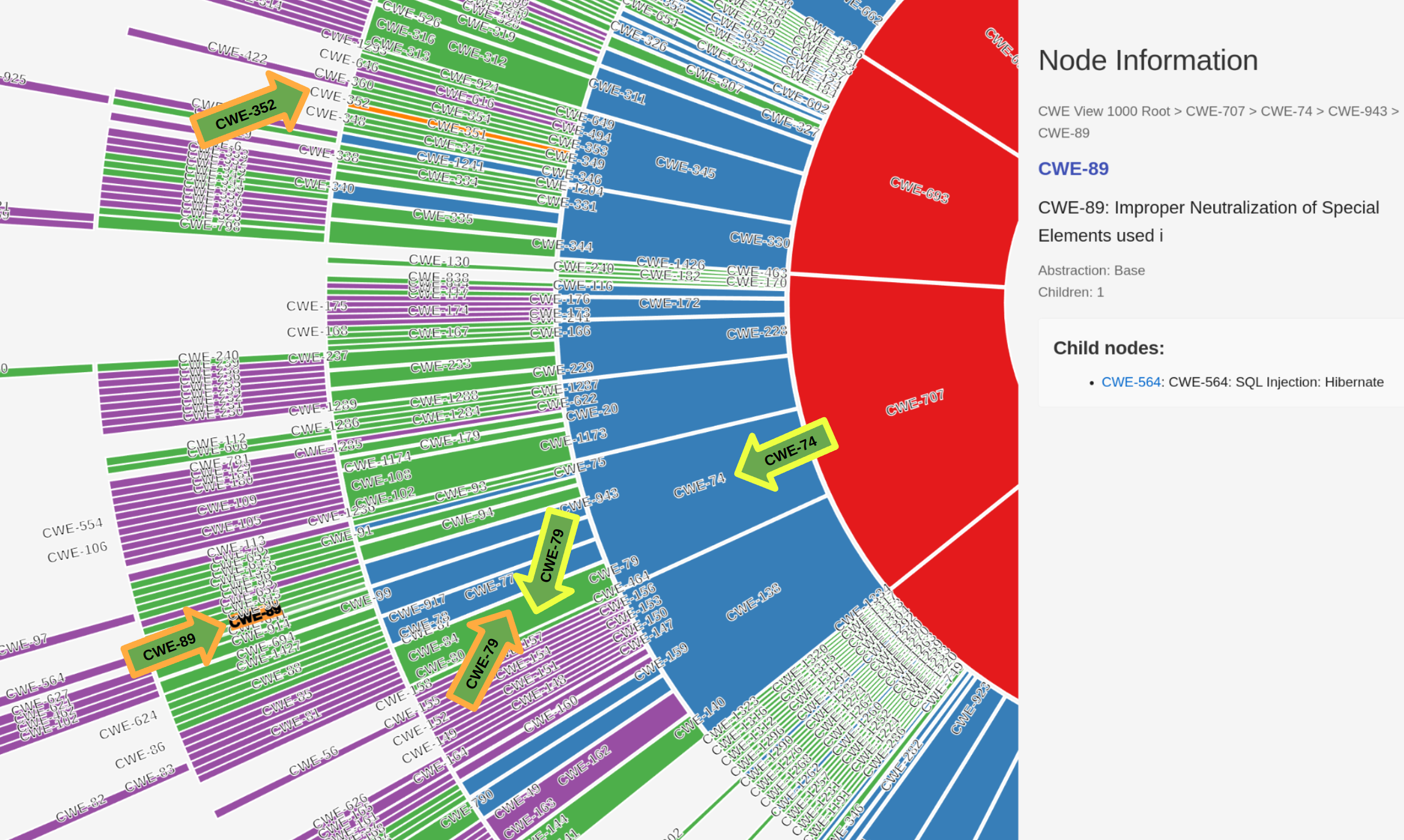
✅ CWE-79 was correctly assigned
❓ CWE-89 was assigned. This is more specific than CWE-74
- Is this wrong or more right?
- Does this get partial credit or no credit?
❌ CWE-352 was incorrectly assigned
- Is there a penalty for a wrong guess?

Similarly, how would we score it for

Benchmark: CWE-79, CWE-89, CWE-352
Prediction: CWE-79, CWE-74

Question

Do we reward proximity? i.e. close but not exactly the Benchmark CWE(s).

What View determines proximity? e.g. View-1003, View-1000.

Do we penalize wrong? i.e. far from any Benchmark CWE(s).

Are classification errors in the upper levels of the hierarchy (e.g. when wrongly classifying a CWE in the wrong pillar) more severe than those in deeper levels (e.g. when classifying a CVE from Base to Variant)

Do we reward specificity? i.e. for 2 CWEs in proximity to the Benchmark CWE(s), do we reward a more specific CWE(s) versus a more general CWE(s)?

Benchmark CWE View Selection¶

Info

The most specific accurate CWE should be assigned to a CVE i.e. not limited by views which contain a subset of CWEs e.g. View-1003.

Therefore, the benchmark should support all CWEs

Tip

Research View (View-1000) will be used as the CWE View to base benchmark scoring on.

See details on different views and why Research View (View-1000) is the best view to use.

Benchmark Scoring Algorithm¶

This section is an overview of different CWE benchmarking scoring approaches.

Data Points¶

Info

A CVE can have one or more CWEs i.e. it's a multi-label classification problem.

MITRE CWE list is a rich document containing detailed information on CWEs (~2800 pages).

The RelatedNatureEnumerations form a (view-dependent e.g. CWE-1000) Directed Acyclic Graph (DAG)

1309 ChildOf/ParentOf
141 CanPrecede/CanFollow
13 Requires/RequiredBy

CVE info (Description and References) may lead to some ambiguity as to the best CWE.

Scoring System: Overview¶

The goal is to assign a numeric score that:

Rewards exact matches highly.
Rewards partial matches based on hierarchical proximity (parent-child relationships).
Penalizes wrong assignments.
Provides a standardized range (e.g. 0 to 1) for easy comparison.
Is based on the CWE hierarchy.
Reinforces good mapping behavior.

Definitions & Assumptions¶

Ground Truth (Benchmark): One or more known-good CWEs per CVE.
Prediction: One or more CWEs assigned by the tested solution.
Hierarchy: Relationships defined by MITRE’s CWE hierarchy (RelatedNatureEnumerations).
Proximity: Measured as shortest hierarchical path (edge distance) between two CWEs for a given View.
- If there is more than one path, the Primary Path is used.

Interesting Cases¶

Evaluation Measures for Hierarchical Classification: a unified view and novel approaches, June 2013, presents the interesting cases when evaluating hierarchical classifiers.

Scoring Approaches¶

The following Scoring Approaches are detailed:

Path Based using CWE graph distance based on ChildOf
1. Path based Proposal
2. See Critique
Hierarchical Classification Standards
1. A survey of Hierarchical Classification Standards
2. A proposal with Worked Examples

Tip

Hierarchical Classification Standards look the most promising.

Shortest Path¶

Step-by-Step Scoring Methodology¶

Step 1: Calculate Hierarchical Distance¶

For each predicted CWE, calculate the shortest distance to each benchmark CWE:

Exact match: Distance = 0
Direct Parent or Child: Distance = 1
Grandparent, Grandchild, or Sibling: Distance = 2
Greater Distance (up/down the tree): Increment by 1 per hierarchical level traversed

If no hierarchical path exists between CWEs (unrelated), assign a large default penalty (e.g., distance = 10).

Step 2: Convert Distances to Proximity Scores¶

Convert hierarchical distances into proximity scores. For example:

$ProximityScore(d) = \frac{1}{(1 + d)}$

This formula produces intuitive scores:

Distance	Proximity Score
0	1.00
1	0.50
2	0.33
3	0.25
4	0.20
≥10	~0.09 or lower

Step 3: Aggregate Proximity Scores (Multi-label Case)¶

Because a CVE can have multiple benchmark CWEs and multiple predictions, aggregate as follows:

For each predicted CWE, take the average (or sum normalized by number of benchmarks) of proximity scores across all benchmark CWEs.

Given:

Benchmark CWEs:

\[ \text{Benchmark CWEs B}= \{b_1, b_2, \dots, b_m\} \]

Predicted CWEs:

\[ \text{Predicted CWEs P}= \{p_1, p_2, \dots, p_n\} \]

Evaluation Metrics¶

Recall¶

Evaluate how well benchmark CWEs are covered by predictions:

\[ \text{Recall}_{CVE} = \frac{1}{|B|} \sum_{b \in B} \left( \frac{\sum_{p \in P} \text{ProximityScore}(b, p)}{|P|} \right) \]

Precision¶

Evaluate how accurately predictions align with benchmark CWEs:

\[ \text{Precision}_{CVE} = \frac{1}{|P|} \sum_{p \in P} \left( \frac{\sum_{b \in B} \text{ProximityScore}(p, b)}{|B|} \right) \]

F1-Score¶

Harmonic mean of precision and recall:

\[ \text{F1}_{CVE} = \frac{2 \times \text{Precision}_{CVE} \times \text{Recall}_{CVE}}{\text{Precision}_{CVE} + \text{Recall}_{CVE}} \]

Worked Example¶

Benchmark CWEs: CWE-79, CWE-89
Predicted CWEs: CWE-79, CWE-74 (distance 2 from CWE-79, distance 3 from CWE-89), CWE-352 (unrelated)

Predicted CWE	Benchmark CWE	Distance $ d $	Proximity Score
CWE-79	CWE-79	0	1.00
CWE-79	CWE-89	3	0.25
CWE-74	CWE-79	2	0.33
CWE-74	CWE-89	3	0.25
CWE-352	CWE-79	10	0.09
CWE-352	CWE-89	10	0.09

Recall Calculation:¶

$$ \text{Recall (CWE-79)} = \frac{1.00 + 0.33 + 0.09}{3} = 0.473 $$

$$ \text{Recall (CWE-89)} = \frac{0.25 + 0.25 + 0.09}{3} = 0.197 $$

$$ \text{Overall Recall} = \frac{0.473 + 0.197}{2} = 0.335 $$

Precision Calculation:¶

$$ \text{Precision (CWE-79)} = \frac{1.00 + 0.25}{2} = 0.625 $$

$$ \text{Precision (CWE-74)} = \frac{0.33 + 0.25}{2} = 0.29 $$

$$ \text{Precision (CWE-352)} = \frac{0.09 + 0.09}{2} = 0.09 $$

$$ \text{Overall Precision} = \frac{0.625 + 0.29 + 0.09}{3} = 0.335 $$

F1-Score Calculation:¶

\[ \text{F1-score} = \frac{2 \times 0.335 \times 0.335}{0.335 + 0.335} = 0.335 \]

Interpretation¶

Scores near $1.0$ indicate highly accurate assignments.
Scores around $0.3 - 0.5$ indicate moderate accuracy.
Lower scores indicate poor predictions.

Topics Not Covered¶

Assign different weights to different relationship types:
- ChildOf/ParentOf: Weight 1.0
- Requires/RequiredBy: Weight 0.8
- CanPrecede/CanFollow: Weight 0.7
- Sibling Of (same parent): Weight 0.6
Introduce a tunable parameter B to adjust the sensitivity of proximity scores:

\[ \text{ProximityScore}(d) = \frac{1}{1 + \beta \times d} \]

Comparative Analysis of a Proposed Hierarchical Scoring Formula against Research Findings for CWE Classification Evaluation¶

1. Introduction¶

1.1. Context¶

The CWE structure is inherently hierarchical, typically represented as a Directed Acyclic Graph (DAG), where weaknesses are organized into different levels of abstraction (e.g., Pillar, Class, Base, Variant).

Furthermore, a single CVE can often be associated with multiple CWEs, reflecting different facets of the underlying vulnerability. Consequently, the evaluation of automated CWE assignment tools falls under the domain of Hierarchical Multi-label Classification (HMC).

1.2. Problem Statement¶

Evaluating HMC systems necessitates metrics that go beyond traditional flat classification measures.

Standard metrics like accuracy, precision, and recall, when applied naively, often fail to account for the crucial aspects of HMC: the hierarchical relationships between classes and the multi-label nature of predictions.
Ignoring the hierarchy means treating all classification errors as equally severe, which contradicts intuition; for instance, misclassifying a specific type of 'Cross-Site Scripting' (a deep node) as a different specific type might be considered less erroneous than misclassifying it as 'Improper Access Control' (a node in a completely different branch, potentially shallower).
Similarly, standard multi-label metrics might not adequately incorporate the hierarchical structure when assessing partial correctness. Therefore, specialized evaluation measures are required for meaningful assessment and comparison of HMC algorithms.

1.3. Shortest Path Proposal Overview¶

This report analyzes a proposed scoring formula designed for evaluating automated CWE classification systems. The formula attempts to address the HMC nature of the task by incorporating a measure of distance within the CWE hierarchy to calculate a proximity score, which is then used to compute custom Precision, Recall, and F1-score metrics, aggregated across multiple labels and instances.

1.4. Report Objectives and Structure¶

The primary objective of this report is to provide an expert analysis of the proposed scoring formula, comparing its components and overall methodology against established research findings and best practices in HMC evaluation, particularly within the context of CWE classification. This analysis will identify the strengths and weaknesses of the proposal and offer concrete, research-backed recommendations for improvement. The report is structured as follows:

Section 2 dissects the components of the formula.
Section 3 compares the proposed hierarchical distance metric against alternatives discussed in the research.
Section 4 evaluates the proposed aggregation method for Precision and Recall relative to standard multi-label and hierarchical practices.
Section 5 assesses the partial credit mechanism.
Sections 6 and 7 summarize the pros and cons of the proposal, respectively.
Section 8 analyzes the potential impact of the suggested future work ("Topics Not Covered" items).
Section 9 proposes specific improvements based on the research.
Finally, Section 10 provides concluding remarks.

2. Analysis of the Proposed Scoring Formula¶

The proposed formula consists of three main components: a method for calculating hierarchical distance, a function to convert this distance into a proximity score, and an aggregation method to compute overall Precision, Recall, and F1-score.

2.1. Hierarchical Distance Calculation¶

The core of the hierarchical component relies on calculating the distance between a predicted CWE node and a true CWE node within the hierarchy graph.

Method: The proposed distance metric is the Shortest Path Length (SPL) between the two nodes in the CWE hierarchy graph. The CWE hierarchy is generally structured as a Directed Acyclic Graph (DAG), allowing multiple parents for a node. The SPL calculation presumably traverses the graph edges, counting the number of steps in the shortest path connecting the two nodes, ignoring edge directionality for distance calculation purposes.
Sibling/Unrelated Handling: For cases where nodes do not lie on a direct ancestor-descendant path, the proposal introduces specific, fixed distance values. If two nodes are siblings (sharing an immediate parent), a distance $d_{sibling}$ is assigned. If nodes are otherwise unrelated (no shared parent and not in an ancestor/descendant relationship, potentially only sharing the root or very distant ancestors), a distance $d_{unrelated}$ is assigned. These appear to be user-defined parameters.
Implicit Assumptions: This method implicitly assumes that each edge in the CWE hierarchy represents a uniform semantic distance, typically a distance of 1. It does not differentiate between different types of relationships (e.g., ParentOf, ChildOf, MemberOf, PeerOf mentioned in CWE documentation) or the level of abstraction at which the relationship occurs.

2.2. Proximity Score Conversion¶

The calculated distance $d$ is then transformed into a proximity score $s$ using an inverse relationship.

Formula: The conversion uses the formula $s = 1 / (1 + d)$.
Behavior: This function maps distances to a score between 0 and 1. When the distance $d=0$ (i.e., the predicted node is the same as the true node), the score $s=1$. As the distance $d$ increases, the score $s$ decreases non-linearly, approaching 0 for very large distances. This provides an intuitive mapping where closer nodes in the hierarchy receive higher proximity scores.
Partial Credit Mechanism: This score $s$ serves as the mechanism for awarding partial credit. A prediction that is incorrect ($d>0$) but hierarchically close to a true label still receives a score greater than 0, reflecting partial correctness. The amount of credit decreases as the hierarchical distance increases.

2.3. Aggregation for Precision/Recall/F1¶

The final step involves aggregating these proximity scores to calculate overall Precision (P), Recall (R), and F1-score (F1) for the classification task, considering the multi-label nature.

Method: The proposal outlines a custom aggregation method. While the exact details require clarification, it appears to involve summing the proximity scores ($s$) calculated between pairs of predicted and true labels for each data instance (e.g., a CVE). These summed scores are then likely normalized in some way to produce example-level P, R, and F1 values.
Example-Level Calculation: For a single CVE with a set of true CWEs $Y=\{y_1,...,y_N\}$ and a set of predicted CWEs $P=\{p_1,...,p_M\}$, the calculation likely involves computing the proximity score $s_{ij} = 1 / (1 + d(p_i, y_j))$ for relevant pairs $(p_i, y_j)$. How these pairwise scores are combined into example-level P and R is crucial but unspecified – it might involve averaging scores for each predicted label against all true labels (for P) or for each true label against all predicted labels (for R), potentially using maximums or sums. For instance, a possible interpretation for example-level Precision could be $\frac{1}{M} \sum_{i=1}^{M} \max_{j=1}^{N} s_{ij}$ and for Recall $\frac{1}{N} \sum_{j=1}^{N} \max_{i=1}^{M} s_{ij}$, although other summation or averaging schemes are possible.
Overall Aggregation: The example-level P, R, and F1 scores are then aggregated across the entire dataset to produce the final metrics. The proposal suggests simple averaging of these example-level scores, which corresponds to a form of macro-averaging, but applied to custom, non-standard example-level metrics.

3. Comparison of the Proposed Hierarchical Distance Metric¶

The choice of a distance or similarity metric is fundamental to incorporating hierarchical information into the evaluation. The proposal utilizes Shortest Path Length (SPL), which needs to be compared against metrics discussed in the research literature.

3.1. Comparison with Path-Length Based Metrics¶

Path-length based metrics are a common starting point for measuring similarity in ontologies and hierarchies.

User Proposal (SPL): The proposal uses the direct shortest path length between nodes.
Research Findings (Pros): The primary advantage of SPL is its simplicity and intuitive appeal: nodes that are fewer steps apart in the graph are considered more similar. It is computationally straightforward to calculate using standard graph traversal algorithms like Breadth-First Search. SPL forms the basis for several established semantic similarity measures.
Research Findings (Cons): Despite its simplicity, SPL suffers from significant drawbacks when used for semantic similarity in rich hierarchies:
- Ignoring Node Depth/Specificity: SPL treats all edges as equal, regardless of their depth in the hierarchy. However, nodes deeper in a hierarchy typically represent more specific concepts. An edge connecting two general concepts near the root (e.g., 'Hardware Fault' to 'Software Fault') often represents a larger semantic distance than an edge connecting two specific concepts deep within a branch (e.g., 'Off-by-one Error' to 'Buffer Overflow'). SPL fails to capture this crucial aspect of semantic specificity tied to depth. Research emphasizes the importance of considering node depth and the depth of the Least Common Subsumer (LCS) – the deepest shared ancestor – for more meaningful similarity assessment.
- Uniform Edge Weights: The assumption of uniform distance (cost=1) for every edge is often unrealistic. The semantic distance between a parent and child might vary across the hierarchy, or different relationship types (if present beyond parent/child) might imply different distances. The SPL metric inherently adopts this uniformity assumption.
- Arbitrary Sibling/Unrelated Values: Assigning fixed, arbitrary values like $d_{sibling}$ and $d_{unrelated}$ lacks a principled foundation. Standard path-based measures often focus on ancestor-descendant relationships or paths through the LCS, implicitly treating unrelated nodes as infinitely distant or requiring specific handling based on the LCS. The approach makes the final score highly sensitive to these parameters, whose values are not derived from the hierarchy's structure or semantics.

3.2. Comparison with Other Semantic Similarity Metrics¶

Recognizing the limitations of simple path length, researchers have developed more sophisticated metrics:

Wu & Palmer Similarity: This widely cited measure directly addresses the depth issue. Its formula, $$ Sim_{WP}(c_1, c_2) = \frac{2 \times depth(LCS(c_1, c_2))}{depth(c_1) + depth(c_2)} $$ incorporates the depth of the two concepts ($c_1, c_2$) and their Least Common Subsumer (LCS). By considering the depth of the LCS relative to the depths of the concepts themselves, it provides a measure of similarity that accounts for specificity. Concepts sharing a deeper LCS are considered more similar. While popular, it can sometimes produce counter-intuitive results depending on the ontology structure.
LCS Depth: A simpler approach related to Wu & Palmer is to use the depth of the LCS itself as a similarity indicator: the deeper the LCS, the more specific the shared information, and thus the higher the similarity.
Information Content (IC) Based Measures: These methods quantify the specificity of a concept based on its probability of occurrence in a corpus or its structural properties within the ontology (e.g., number of descendants). Common IC-based similarity measures (e.g., Resnik, Lin, Jiang & Conrath) typically use the IC of the concepts and their LCS. For example, Resnik similarity is simply the IC of the LCS. These measures can capture data-driven or structure-driven semantics effectively but depend on the availability of a suitable corpus or a well-structured ontology.

The choice of SPL prioritizes topological proximity over the semantic nuances captured by depth, specificity, and information content. While simpler to compute, SPL may fail to accurately reflect the semantic relatedness between CWEs, potentially leading to misleading evaluations where errors between semantically distant but topologically close nodes are penalized less than errors between semantically closer but topologically more distant nodes. Metrics like Wu & Palmer or IC-based approaches are generally considered more semantically grounded for hierarchical evaluation.

3.3. Relevance to CWE Hierarchy¶

The specific characteristics of the CWE hierarchy further challenge the suitability of simple SPL.

Structure: CWE is organized as a DAG, not strictly a tree, meaning nodes can have multiple parents. It features multiple levels of abstraction (Pillar, Class, Base, Variant) representing different granularities of weaknesses. The hierarchy is also actively maintained and evolves.
Challenges for SPL: The DAG structure means multiple paths may exist between nodes; SPL typically uses only the shortest, potentially ignoring semantically meaningful connections. The defined abstraction levels strongly imply non-uniform semantic distances between parent-child pairs across different levels, which SPL ignores. For example, the semantic jump from a Pillar to a Class might be larger than from a Base to a Variant.
Mapping Practices: The National Vulnerability Database (NVD) and others mapping CVEs to CWEs sometimes use higher-level CWEs or map to specific "views" like View-1003 (a simplified mapping) for consistency or due to ambiguity. This practice complicates evaluation: if the ground truth is a specific 'Base' level CWE (e.g., CWE-787 Out-of-bounds Write), is predicting its 'Class' level parent (e.g., CWE-119 Improper Restriction of Operations within the Bounds of a Memory Buffer) partially correct? The metric assigns partial credit via $1/(1+d)$, but the amount is based solely on path length, not the semantic relationship or abstraction level difference. Metrics sensitive to depth and structure, or methods like set-augmentation (discussed later), might handle these nuances more appropriately.

4. Evaluation of the Proposed Aggregation Method¶

The method used to aggregate scores across multiple labels and instances is critical for producing meaningful overall performance metrics. The proposal employs a custom aggregation based on summed proximity scores, which needs comparison with standard practices.

4.1. Contrast with Standard Multi-Label Metrics¶

Standard evaluation in multi-label classification employs several well-defined metrics:

User Proposal: A custom P/R/F1 calculation based on summing $1/(1+d)$ proximity scores, likely averaged at the example level first.
Standard Metrics: These are broadly categorized:
- Example-Based Metrics: Evaluate performance on an instance-by-instance basis. Key examples include:
  - Subset Accuracy (Exact Match Ratio): The strictest metric; requires the predicted set of labels to exactly match the true set. Score is 1 if identical, 0 otherwise. It gives no partial credit.
  - Hamming Loss: The fraction of labels that are incorrectly predicted (misclassifications + missed labels), averaged over instances. Lower is better. It treats all labels and errors equally.
  - Example-Based P/R/F1: Calculates precision, recall, and F1 for each example based on the intersection and union of predicted and true label sets (e.g., using Jaccard similarity for F1: $|P \cap Y| / |P \cup Y|$). Then averages these scores across examples.
- Ranking Metrics: Treat the output as a ranked list of labels. Examples include Ranking Loss, Average Precision, and One-Error. These are useful when the order or confidence of predictions matters.
- Label-Based (Averaging) Metrics: Adapt binary metrics (P/R/F1) to the multi-label setting by averaging across labels. The two main approaches are Micro and Macro averaging.

4.2. Micro vs. Macro Averaging¶

Micro and Macro averaging are standard ways to aggregate P/R/F1 scores in multi-class and multi-label settings:

Definitions:
- Micro-average: Aggregates the counts of True Positives (TP), False Positives (FP), and False Negatives (FN) across all classes/labels first. Then computes the metric (e.g., Precision = $\sum TP / (\sum TP + \sum FP)$) from these global counts.
- Macro-average: Calculates the metric (e.g., Precision) independently for each class/label. Then computes the simple arithmetic mean of these per-class metrics.
Interpretability:
- Micro-average: Gives equal weight to each classification decision (or each instance in multi-label settings where metrics are computed per instance). It reflects overall performance across all predictions. In multi-class (single-label per instance) settings, Micro-F1 equals Accuracy.
- Macro-average: Gives equal weight to each class/label, regardless of its frequency. It reflects the average performance across all classes.
Sensitivity to Imbalance: This difference in weighting is crucial for imbalanced datasets, which are common in HMC. Micro-average scores are dominated by the performance on the majority classes. Macro-average scores treat rare classes and frequent classes equally, making it a better indicator of performance across the board, especially for identifying weaknesses in classifying minority classes. Weighted macro-averaging, which weights each class's metric by its support (number of true instances), offers a compromise.

The proposed aggregation method, likely averaging custom example-level scores, resembles Macro-averaging in spirit but applies it to non-standard base metrics. This lack of grounding in the standard TP/FP/FN counts used by Micro/Macro averaging makes the resulting values difficult to interpret statistically, especially regarding their behavior with class imbalance. It is unclear whether the metric reflects overall decision accuracy (like Micro) or average per-class performance (like Macro).

4.3. Contrast with Hierarchical Aggregation (hP/hR/hF)¶

To explicitly incorporate hierarchy into P/R/F1, the set-augmentation approach leading to hierarchical Precision (hP), Hierarchical Recall (hR), and Hierarchical F-measure (hF) is a recognized standard.

Set-Augmentation (hP/hR/hF): This approach modifies the sets of true labels (Y) and predicted labels (P) for a given instance before calculating standard P/R/F1. Both sets are augmented by adding all their respective ancestor nodes in the hierarchy. Let $An(c)$ be the set of ancestors of class $c$. Augmented true set: $$ Y_{aug} = Y \cup \bigcup_{y \in Y} An(y) $$ Augmented predicted set: $$ P_{aug} = P \cup \bigcup_{p \in P} An(p) $$ Hierarchical Precision: $$ hP = \frac{|P_{aug} \cap Y_{aug}|}{|P_{aug}|} $$ Hierarchical Recall: $$ hR = \frac{|P_{aug} \cap Y_{aug}|}{|Y_{aug}|} $$ Hierarchical F-measure: $$ hF = \frac{2 \times hP \times hR}{hP + hR} $$
Averaging hP/hR/hF: These example-wise hierarchical metrics are then typically aggregated across the dataset using standard Micro or Macro averaging. This yields metrics like Micro-hF and Macro-hF, which combine hierarchical awareness (via set augmentation) with standard, interpretable aggregation methods.

Comparison: The hP/hR/hF approach integrates the hierarchy by redefining what constitutes a relevant prediction (considering ancestors), but then applies the standard, well-understood definitions of P/R based on set intersections and cardinalities. The method, conversely, keeps the notion of prediction sets standard but defines custom P/R based on summed, distance-derived proximity scores. The hP/hR/hF approach is arguably more integrated with the established evaluation framework.

4.4. Interpretability of P/R Metrics¶

A major drawback of the proposal is the lack of clear interpretability of the resulting P/R/F1 scores.

Lack of Standard Meaning: Standard Precision represents the probability that a positive prediction is correct; standard Recall represents the probability that a true positive instance is correctly identified. It is unclear what probabilistic or set-theoretic meaning can be ascribed to the metrics derived from summing $1/(1+d)$ scores. A score of, say, 0.7 for the "Precision" cannot be directly interpreted in the same way as a standard Precision score of 0.7.
Sensitivity: The scores are sensitive to the specific distance function ($d$) and the transformation ($s=1/(1+d)$). The choice of arbitrary distances $d_{sibling}$ and $d_{unrelated}$ can significantly impact the final score without a clear semantic justification. The non-linear decay of the proximity score also influences how errors at different distances contribute to the sum.
Comparability Issues: The use of non-standard, custom metrics severely hinders comparability with other research and benchmark results. Established metrics like Micro-F1, Macro-F1, Micro-hF, and Macro-hF serve as common ground for evaluating HMC systems. Results based on the proposed custom metrics cannot be readily compared, making it difficult to assess relative performance or progress.

5. Assessment of the Partial Credit Mechanism¶

A key motivation for hierarchical evaluation is to award partial credit for predictions that are incorrect but "close" in the hierarchy.

5.1. User Proposal: Proximity Score $1/(1+d)$¶

Mechanism: The formula $s=1/(1+d)$ directly implements a continuous partial credit scheme. The closer the prediction (smaller $d$), the higher the score $s$ (approaching 1), and vice versa. Credit diminishes non-linearly with distance.
Nature: Explicit, continuous, distance-based partial credit.

5.2. Research Standard: Set-Augmentation (hP/hR/hF)¶

Mechanism: The hP/hR/hF measures provide partial credit implicitly through the set augmentation process. When calculating the intersection $|P_{aug} \cap Y_{aug}|$, a predicted node $p$ contributes positively if it, or one of its ancestors, matches a true node $y$ or one of its ancestors. Predicting a parent, grandparent, or even a sibling (if they share a close common ancestor included in the augmented sets) of a true label can result in a non-zero intersection, thus contributing to the hP and hR scores.
Nature: Implicit, set-overlap based partial credit, grounded in shared hierarchical context.

5.3. Comparison¶

Granularity: The method provides a seemingly finer-grained partial credit score based on the exact distance value $d$. The hP/hR/hF mechanism is based on set membership overlap; the contribution to the intersection size is effectively binary for each element in the augmented sets, but the overall score reflects the degree of overlap.
Penalty for Large Errors: How severely are very distant errors penalized? In the method, $s=1/(1+d)$ approaches zero as $d$ increases but never reaches it unless $d$ is infinite. This might assign small amounts of credit even to predictions that are semantically very far away, depending on the scale of $d$ and the values chosen for $d_{unrelated}$. In the hP/hR/hF approach, if a predicted node $p$ and a true node $y$ share no ancestors other than perhaps the root (which might be excluded from augmentation depending on the implementation), their augmented sets $An(p) \cup \{p\}$ and $An(y) \cup \{y\}$ might have minimal or no overlap. In such cases, the incorrect prediction $p$ contributes nothing towards matching $y$ in the intersection calculation, effectively receiving zero credit relative to that specific true label. This aligns with the intuition that grossly incorrect predictions should be heavily penalized. The $1/(1+d)$ function's decay might not be steep enough to adequately penalize such errors.
Interpretability: The partial credit in hP/hR/hF arises naturally from applying the standard P/R definitions to hierarchically augmented sets. It fits within the well-understood framework of true positives, false positives, and false negatives, albeit defined over augmented sets. The $1/(1+d)$ score, while intuitive as a concept ("closer is better"), is an ad-hoc value whose contribution to the final non-standard P/R metrics lacks a clear, established interpretation within classification evaluation theory.

While the continuous score appears nuanced, the set-augmentation method integrates partial credit more coherently with the standard Precision/Recall framework, offering better interpretability and likely a more appropriate handling of severe errors.

6. Summary of Pros of the Proposal¶

Despite its limitations when compared to established research methods, the proposed formula exhibits several positive attributes:

Acknowledges Hierarchy: The proposal explicitly recognizes the hierarchical nature of the CWE classification task and attempts to incorporate this structure into the evaluation, moving beyond inadequate flat classification metrics.
Handles Multi-Label: The design considers the multi-label aspect, where a single CVE can map to multiple CWEs, aiming to evaluate predictions against potentially multiple true labels.
Intuitive Proximity Score: The conversion of distance $d$ to a proximity score $s$ via $s=1/(1+d)$ is conceptually straightforward and aligns with the intuition that predictions closer in the hierarchy are better than those farther away.
Provides Partial Credit: Unlike strict metrics like Subset Accuracy, the formula incorporates a mechanism for awarding partial credit, acknowledging that some incorrect predictions are "less wrong" than others based on hierarchical proximity.
Simplicity (Distance Metric): The use of Shortest Path Length (SPL) as the distance metric is computationally simple and easy to implement compared to more complex semantic similarity measures that might require external corpora or intricate structural analysis.

7. Summary of Cons of the Proposal¶

The proposed formula suffers from several significant drawbacks when evaluated against established HMC evaluation principles and research findings:

Simplistic Distance Metric: The core SPL distance metric ignores crucial semantic information embedded in the hierarchy, such as node depth (specificity) and the varying semantic distances between different levels of abstraction. Treating all hierarchical links as having uniform weight is a major oversimplification for complex taxonomies like CWE.
Arbitrary Parameters: The reliance on user-defined, fixed distance values for sibling ($d_{sibling}$) and unrelated ($d_{unrelated}$) nodes introduces arbitrariness. The metric's behavior becomes sensitive to these parameters, which lack a clear theoretical or empirical justification.
Non-Standard Aggregation: The custom method for calculating Precision, Recall, and F1-score based on summing proximity scores deviates significantly from standard, well-defined aggregation techniques like Micro and Macro averaging.
Unclear Interpretability: The resulting P/R/F1 scores lack a clear statistical or probabilistic interpretation. It is difficult to understand what aspect of performance they truly measure or how they behave under conditions like class imbalance, making them hard to interpret meaningfully.
Comparability Issues: The use of non-standard metrics makes it virtually impossible to compare results obtained using this formula with those from other studies or benchmarks that employ established HMC metrics like hF (Micro/Macro averaged).
Potentially Insufficient Penalty for Large Errors: The gentle decay of the $1/(1+d)$ score might not sufficiently penalize predictions that are hierarchically very distant from the true labels, potentially inflating scores compared to methods like hP/hR/hF where such errors contribute minimally or not at all to the positive counts.
Ignores Edge Weights/Types: The underlying SPL assumes uniform edge weights and doesn't account for potentially different relationship types within the CWE structure, further limiting its semantic accuracy.

8. Analysis of "Topics Not Covered" Items¶

The user identified two potential areas for future improvement: weighting relationships and incorporating a beta parameter in the F-score.

8.1. Weighting Relationships¶

User Intent: This suggestion aims to address the limitation of assuming uniform distance for all hierarchical links by assigning different weights based on the relationship type (e.g., parent-child vs. sibling) or potentially the depth.
Research Context: This aligns with the critique of basic path-based measures that treat all edges equivalently. More advanced graph-based semantic measures sometimes incorporate edge weighting schemes.
Evaluation: Introducing weights is a step towards acknowledging non-uniform semantic distances. However, applying weights to a simple SPL calculation still does not fundamentally address the more critical issue of ignoring node depth and specificity, which metrics like Wu & Palmer or IC-based measures handle more directly. Furthermore, it introduces additional parameters (the weights themselves) that require careful justification and tuning, potentially adding complexity without guaranteeing a more semantically sound metric compared to established alternatives like Wu & Palmer or the set-augmentation approach. It refines the SPL approach but doesn't replace it with a more robust foundation.

8.2. Beta Parameter in F-Score¶

User Intent: The proposal suggests incorporating a beta parameter, presumably to create an F-beta score analogous to the standard definition: $$ F_\beta = \frac{(1 + \beta^2) \times P \times R}{(\beta^2 \times P) + R} $$ This allows tuning the F-score to prioritize either Precision ($\beta<1$) or Recall ($\beta>1$).
Research Context: Using the F-beta score is a standard technique in classification evaluation when there is an asymmetric cost associated with false positives versus false negatives, or a specific need to emphasize either precision or recall.
Evaluation: While incorporating a beta parameter is standard practice for balancing P and R, its utility depends entirely on the meaningfulness of the underlying P and R metrics. Applying it to the custom, non-standard P and R values does not fix the core problems associated with their calculation and interpretation. The fundamental issues lie in the distance metric and the aggregation method used to derive P and R, not in how they are combined into an F-score. Improving the P and R calculations themselves is far more critical than allowing for a beta-weighted combination of potentially flawed metrics.

8.3. Addressing Core Limitations?¶

The proposed "Topics Not Covered" items demonstrate an awareness of some of the formula's limitations, specifically the uniform edge weight assumption and the fixed balance of the F1 score.

However, they represent incremental adjustments to the existing framework rather than a shift towards fundamentally different, research-backed methodologies. They fail to address the core weaknesses identified in Sections 3 and 4: the semantic inadequacy of the SPL distance metric (ignoring depth/specificity) and the non-standard, uninterpretable aggregation method for P/R/F1.

Therefore, implementing these suggestions would likely yield only marginal improvements and would not resolve the fundamental issues of interpretability, comparability, and semantic relevance compared to established HMC evaluation practices.

9. Proposed Improvements Based on Research¶

Based on the analysis and comparison with established HMC evaluation research, the following improvements are recommended to create a more robust, interpretable, and comparable evaluation framework for the CWE classification task.

9.1. Adopt Standard Hierarchical Metrics (hP/hR/hF)¶

Recommendation: Replace the custom P/R/F1 calculations based on proximity scores with the standard Hierarchical Precision (hP), Hierarchical Recall (hR), and Hierarchical F-measure (hF).
Rationale: These metrics are specifically designed for HMC. They incorporate the hierarchy through set augmentation (adding ancestors to true and predicted sets) and then apply the standard, well-understood definitions of precision and recall based on the intersection and cardinality of these augmented sets. This approach provides inherent partial credit for predictions that share hierarchical context (ancestors) with the true labels. It directly addresses the need for hierarchy-aware evaluation within a standard P/R framework, overcoming the interpretability issues of the custom scores. These metrics are increasingly used in HMC literature, facilitating comparison.

9.2. Employ Standard Aggregation Techniques (Micro/Macro Averaging)¶

Recommendation: Calculate the example-wise hP, hR, and hF scores derived from set augmentation. Then, aggregate these scores across the entire dataset using both Micro-averaging and Macro-averaging. Report both Micro-hF and Macro-hF.
Rationale: Micro and Macro averages provide distinct and valuable perspectives on performance. Micro-hF reflects the overall performance weighted by individual predictions, while Macro-hF reflects the average performance per class, treating all classes equally. Reporting both is crucial for understanding performance on potentially imbalanced datasets like CWE, where performance on rare but critical CWEs might be obscured by Micro-averages but highlighted by Macro-averages. Using these standard aggregation methods ensures results are interpretable and comparable to other studies.

9.3. Consider More Robust Distance/Similarity Metrics (If Needed for Other Purposes)¶

Recommendation: If a distance or similarity measure is needed for purposes beyond the primary P/R/F evaluation (e.g., as part of a loss function during model training, or for specific error analysis), replace SPL with a metric that better captures semantic similarity within the hierarchy.
Options:
- Wu & Palmer Similarity: Incorporates node depth and LCS depth, offering a good balance between structural information and computational feasibility. Requires access to the hierarchy structure and node depths.
- LCS-based Measures: Focus on the properties (depth or Information Content) of the Least Common Subsumer, directly measuring shared specificity.
- Information Content (IC) Based Measures: Quantify specificity based on corpus statistics or structural properties (e.g., descendant counts). Can provide strong semantic grounding but require additional data or assumptions about the ontology structure.
Rationale: These metrics address the core limitations of SPL by incorporating information about node depth, specificity, and/or information content, leading to more semantically meaningful comparisons between CWE nodes. The choice among them depends on the specific application requirements and data availability. However, for the primary evaluation metrics, hP/hR/hF based on set augmentation is generally preferred over distance-based aggregation.

9.4. Comparative Summary¶

The following table summarizes the key differences between the proposal and the recommended approach based on hP/hR/hF with standard averaging:

Feature	Proposed Formula	Recommended Approach (hP/hR/hF + Micro/Macro Avg)	Rationale / References
Distance Metric	Shortest Path Length (SPL)	Implicit (via set overlap)	SPL ignores depth/specificity. Set augmentation captures shared hierarchical context.
Partial Credit	Explicit, continuous via $s=1/(1+d)$	Implicit, via overlap of augmented sets ($P_{aug} \cap Y_{aug}$)	Set overlap integrates better with P/R framework, potentially penalizes large errors more appropriately.
Aggregation (P/R)	Custom, sum/average of proximity scores ($s$)	Standard P/R definitions applied to augmented sets ($P_{aug}, Y_{aug}$)	Standard definitions on augmented sets provide clear meaning. method lacks standard interpretation.
Overall Aggregation	Average of custom example-level scores (Macro-like)	Standard Micro- and Macro-averaging of example-level hP/hR/hF	Micro/Macro averages have well-defined interpretations, handle imbalance transparently, ensure comparability.
Interpretability	Low; scores lack standard meaning, sensitive to params	High; based on standard P/R/F1 framework, Micro/Macro well-understood	Standard metrics allow clear interpretation and comparison with literature.
Standardization	Non-standard	Based on established HMC evaluation practices	Adherence to standards is crucial for scientific rigor and comparability.

10. Conclusion¶

This report conducted a comparative analysis of a user-proposed scoring formula for evaluating hierarchical multi-label CWE classification against established research findings and practices. The analysis reveals that while the proposal commendably attempts to incorporate both the hierarchical structure of CWE and the multi-label nature of CVE-to-CWE mapping, it relies on methods that deviate significantly from research-backed standards.

The strengths of the proposal lie in its explicit acknowledgment of the HMC problem, its intuitive mechanism for assigning proximity scores based on distance, and the inclusion of partial credit. However, these are overshadowed by significant weaknesses. The core distance metric, Shortest Path Length, is overly simplistic, ignoring crucial semantic information like node depth and specificity, which are vital in hierarchical contexts. Furthermore, the reliance on arbitrary parameters for sibling/unrelated distances and the custom aggregation method for Precision, Recall, and F1-score result in metrics that lack clear statistical interpretation and are difficult to compare with standard benchmarks. The proposed items, while showing awareness of some limitations, do not address these fundamental issues.

Based on the analysis of relevant research, the recommended approach is to adopt standard HMC evaluation metrics. Specifically, using Hierarchical Precision (hP), Hierarchical Recall (hR), and Hierarchical F-measure (hF) calculated via set augmentation provides a principled way to incorporate the hierarchy and award partial credit within the standard P/R framework. Aggregating these example-wise scores using both Micro- and Macro-averaging ensures interpretable results that account for potential class imbalance and allow for comparison with other studies. If distance-based measures are required for other analyses, metrics like Wu & Palmer similarity offer more semantic richness than simple path length.

Adopting these standard, research-backed evaluation practices will lead to more rigorous, interpretable, and comparable assessments of automated CWE classification systems. While developing novel metrics can be valuable, it is crucial to ensure they are well-grounded theoretically and validated against established methods, particularly in complex evaluation scenarios like HMC. Challenges remain in HMC evaluation, especially concerning the specific complexities of the CWE DAG structure and evolving mapping practices, but leveraging established metrics like hP/hR/hF provides a solid foundation.

11. References¶

A Hierarchical Scoring System for Evaluating Automated CVE-to-CWE Assignments¶

1. Introduction¶

1.1. Problem Statement: Limitations of Traditional Evaluation¶

Evaluating the performance of automated CVE-to-CWE assignment tools presents unique challenges that standard classification metrics fail to adequately address. The complexity arises primarily from two intrinsic characteristics of the CVE-CWE relationship:

Multi-Label Nature: A single CVE does not necessarily map to just one CWE. A specific vulnerability instance (CVE) can arise from the confluence of multiple underlying weaknesses, meaning it may correctly map to a set of CWE identifiers. This multi-label classification scenario invalidates evaluation approaches designed for single-label problems.
Hierarchical Structure: The MITRE CWE list is not a flat collection of independent categories but a structured hierarchy, often represented as a tree or Directed Acyclic Graph (DAG), with defined relationships like parent-child connections. Consequently, prediction errors are not uniform in severity. A predicted CWE that is hierarchically close to a true CWE (e.g., its direct parent or child) represents a more accurate understanding of the weakness than a prediction mapping to a completely unrelated part of the hierarchy. Traditional exact-match evaluation metrics penalize both types of errors equally, failing to capture the nuanced semantic distance between CWEs.

1.2. Objective: Designing the Hierarchical CWE Scoring System (HCSS)¶

The primary objective of this report is to design a Hierarchical CWE Scoring System (HCSS) capable of providing a fair, nuanced, and comprehensive evaluation framework for automated CVE-to-CWE assignment solutions. The HCSS aims to overcome the limitations of traditional metrics by explicitly addressing the multi-label and hierarchical nature of the problem.

The key design requirements for the HCSS are:

Multi-Label Assessment: Accurately evaluate predictions where multiple CWEs can be assigned to a single CVE.
Exact Match Reward: Provide maximum credit for predictions that exactly match the ground-truth CWEs.
Hierarchical Partial Credit: Award partial credit for predicted CWEs that are semantically close to ground-truth CWEs within the MITRE hierarchy.
Penalty for Incorrect Predictions: Appropriately penalize predictions that are unrelated to the true CWEs.
Justifiable Closeness Metric: Incorporate a clearly defined and justifiable metric for quantifying the "closeness" or semantic similarity between CWE nodes.
Robust Aggregation: Provide well-defined methods for aggregating scores, both for individual CVEs and across an entire benchmark dataset.
Grounded Methodology: Base the system on established principles from multi-label classification evaluation, hierarchical classification, and ontology-based semantic similarity measurement.

1.4. Report Roadmap¶

This report systematically addresses the design of the HCSS.

Section 2 examines the relationship between CVEs and CWEs, focusing on the mapping process and its multi-label nature.
Section 3 delves into the structure and semantics of the MITRE CWE hierarchy.
Section 4 discusses the requirements and methods for creating reliable benchmark datasets.
Section 5 reviews standard multi-label and specialized hierarchical classification evaluation metrics.
Section 6 explores various methods for quantifying semantic distance within the CWE hierarchy.
Section 7 analyzes existing practices in evaluating CWE assignment tools and related scoring systems.
Section 8 presents the detailed design of the proposed HCSS, integrating findings from previous sections.
Section 9 provides concluding remarks and suggests directions for future work.
Section 10 links to relevant research.

2. The CVE-CWE Ecosystem: Foundation and Mapping Dynamics¶

Understanding the interplay between CVEs and CWEs, and the processes governing their linkage, is fundamental to designing an appropriate evaluation system.

2.1. Defining CVE and CWE¶

CVE (Common Vulnerabilities and Exposures): Maintained by the MITRE Corporation, CVE serves as a dictionary, providing unique identifiers (CVE IDs) for specific, publicly disclosed cybersecurity vulnerabilities found in software, hardware, or firmware products. Each CVE entry typically includes a standard identifier, a brief description, and references. CVE IDs are assigned by designated organizations known as CVE Numbering Authorities (CNAs), which include vendors, research organizations, and MITRE itself. CVE focuses on cataloging distinct instances of vulnerabilities as they manifest in real-world systems.
CWE (Common Weakness Enumeration): Also managed by MITRE, CWE is a community-developed, formal list or dictionary that categorizes types of weaknesses in software and hardware architecture, design, code, or implementation. These weaknesses represent the underlying flaws or errors that can lead to exploitable vulnerabilities (CVEs). CWE aims to provide a common language for discussing, identifying, and mitigating these root causes, thereby supporting more secure development practices.

Relationship: The relationship between CWE and CVE is often analogized to that between a disease type and a specific patient case. A CWE describes a general category of weakness (e.g., CWE-89: SQL Injection), while a CVE describes a specific instance of that weakness found in a particular product or version (e.g., CVE-2023-12345 describing an SQL injection vulnerability in ExampleApp v1.2). Consequently, CVE records are frequently linked back to one or more CWE entries that represent the fundamental flaws exploited by the vulnerability.

2.2. The CVE-to-CWE Mapping Process¶

The primary public source for CVE-to-CWE mappings is the U.S. National Vulnerability Database (NVD), operated by the National Institute of Standards and Technology (NIST). NVD receives basic CVE information from MITRE and the CNAs and enriches it with additional analysis, including Common Vulnerability Scoring System (CVSS) severity scores, Common Platform Enumeration (CPE) applicability statements identifying affected products, and mappings to relevant CWE identifiers.

However, the mapping process employed by NVD and the broader ecosystem presents several challenges relevant to benchmarking:

Normalization and Specificity Loss: For certain analyses, such as generating the annual CWE Top 25 Most Dangerous Software Weaknesses list, NVD employs a process of "normalization". This involves mapping CVEs primarily to View-1003: Weaknesses for Simplified Mapping of Published Vulnerabilities, a curated subset containing approximately 130 weakness types. If a CVE's initial mapping points to a CWE outside this view, the mapping is often adjusted upwards in the hierarchy to the nearest ancestor within View-1003. While this simplifies analysis for the Top 25 list, it can result in a loss of specificity. A vulnerability accurately identified at a detailed Base or Variant level might be recorded in NVD only at a more general Class or Pillar level. Furthermore, mappings that lack an ancestor within View-1003 may be categorized broadly as "NVD-CWE-Other" or "NVD-CWE-noinfo," or even removed from consideration for certain analyses.
Mapping Quality and Consistency: The accuracy and consistency of mappings can vary. MITRE itself acknowledges that choosing overly high-level CWEs is a common mapping mistake and undertakes efforts to refine mappings, sometimes by consulting the relevant CNAs. CNAs, being closest to the affected products, are often best positioned to provide accurate mappings. However, obtaining feedback from CNAs can be challenging; in one reported re-mapping effort, feedback was received for only 27% of the CVEs submitted for review, leaving the majority with their existing, potentially unverified, mappings.
Ecosystem Stability and Timeliness: The CVE/NVD ecosystem relies on complex workflows and funding structures. Reports have surfaced regarding potential funding expirations for MITRE's operation of the CVE program and backlogs or delays in NVD's enrichment process. Such issues can impact the timeliness, completeness, and potentially the quality of publicly available CVE data, including their associated CWE mappings.

These mapping dynamics carry significant implications for benchmarking. Relying solely on readily available NVD data as ground truth may introduce inaccuracies if the goal is to evaluate a tool's ability to identify the most specific correct CWE. The normalization process means that a tool correctly identifying a Base-level weakness (e.g., CWE-79: Cross-site Scripting) might be unfairly penalized if the benchmark only contains the normalized, higher-level Class mapping (e.g., CWE-74: Improper Neutralization of Special Elements used in an OS Command) derived from View-1003. This potential discrepancy necessitates either careful curation of benchmark datasets to preserve original specificity or designing the scoring system to account for such normalization effects.

Furthermore, the potential for delays or instability in the NVD pipeline highlights the value of static, curated benchmark datasets for reliable and reproducible evaluations. Dependence on live data feeds could introduce variability unrelated to the performance of the tool being assessed. Finally, the variable quality and confidence levels of mappings, stemming from factors like limited CNA review, suggest that benchmark datasets could benefit from documenting the provenance or confidence associated with each ground-truth mapping, potentially allowing for more nuanced evaluation strategies.

2.3. Multi-Label Nature of CVE-CWE Mappings¶

It is explicitly recognized that a single CVE can be associated with multiple CWEs. This reflects the reality that a vulnerability may exploit several distinct types of underlying weaknesses simultaneously. For instance, a vulnerability might involve improper input validation (e.g., CWE-20) leading to the exposure of sensitive information (e.g., CWE-200).

The data structures used for CVEs accommodate this by allowing an array of weakness descriptions (problemtype_data) for each CVE, where each entry can correspond to a different CWE ID.

Descriptions of datasets used for CVE-to-CWE classification research also explicitly frame it as a multi-label classification problem. Therefore, any robust evaluation system must be designed to handle predictions and ground truth represented as sets of CWEs per CVE.

3. Navigating the MITRE CWE Hierarchy: Structure and Semantics¶

The hierarchical organization of the CWE list is central to developing a scoring system that awards partial credit based on semantic closeness. Understanding this structure is therefore essential.

3.1. Hierarchical Structure and Abstraction Levels¶

The CWE hierarchy organizes weakness types into a structure that can be conceptualized as a tree or, more accurately, a Directed Acyclic Graph (DAG), as some weaknesses may have multiple parents. This structure is defined by relationships between CWE nodes and is characterized by several distinct levels of abstraction, providing varying degrees of generality or specificity.

See CWE Relationships.

In addition to these abstraction levels, the CWE content is organized into various Views.

3.2. Relationships Between CWE Nodes¶

The structure of the hierarchy is explicitly defined by several types of relationships connecting CWE nodes (which can be Weaknesses, Categories, or Views).

These relationships allow for systematic navigation of the hierarchy, enabling the identification of ancestors, descendants, parents, children, and peers for any given CWE node. This navigational capability is crucial for calculating hierarchical distances and implementing set-augmentation methods for evaluation.

3.3. Accessing and Interpreting Hierarchy Data¶

The official source for CWE definitions, relationships, and hierarchy structure is the MITRE CWE website. MITRE provides downloadable versions of the CWE list, primarily in XML format. Comprehensive XML downloads encapsulate the entire hierarchy, including weaknesses, categories, views, and their relationships. While CSV downloads are available for specific views, the XML format provides the most complete structural information.

The structure of the XML data is defined by the official CWE XML Schema (XSD), also available from MITRE. This schema details the elements (e.g., <Weakness>, <Category>, <View>), attributes (e.g., ID, Name, Abstraction), and crucially, the elements defining relationships. Hierarchical links like ParentOf and ChildOf are typically represented within a <Related_Weakness> element, which includes attributes specifying the Nature of the relationship (e.g., 'ChildOf', 'ParentOf', 'PeerOf') and the CWE_ID of the related node. Documentation explaining the schema elements is also provided. Various programming libraries and tools can be used to parse and query this XML data to extract the hierarchy structure needed for evaluation.

The explicit definition of abstraction levels offers a direct way to conceptualize hierarchical distance. Moving between adjacent levels (e.g., Variant to Base, Base to Class) represents a discrete step in generality. This structure can be directly leveraged by a closeness metric, perhaps assigning different weights or penalties based on the number of abstraction levels separating two CWEs.

Furthermore, the existence of multiple relationship types (ChildOf, ParentOf, PeerOf, CanAlsoBe) suggests that a sophisticated closeness metric could differentiate based on the type of link, not just its existence or the path length. For instance, ParentOf/ChildOf relationships might imply stronger semantic similarity than PeerOf relationships, reflecting the primary vertical structure of the hierarchy. This nuanced understanding could lead to more accurate partial credit assignments.

Crucially, the availability of the complete hierarchy, including abstraction levels and relationship types, in a machine-readable XML format governed by a defined schema confirms the technical feasibility of implementing an automated scoring system like HCSS. The necessary structural information can be programmatically extracted and utilized for calculating distances and relationships.

4. Benchmark Data for Evaluation: Establishing Ground Truth¶

The reliability and validity of any benchmark depend critically on the quality of the ground truth data used for comparison. For evaluating CVE-to-CWE mapping tools, this requires a "known-good" dataset of CVEs accurately mapped to their corresponding CWE sets.

4.1. Need for a "Known-Good" Benchmark¶

A benchmark dataset serves as the gold standard against which the predictions of automated tools are measured. Its purpose is to provide a consistent, reliable, and representative set of CVE-CWE mappings that reflect the true underlying weaknesses associated with the vulnerabilities. Without such a benchmark, evaluating and comparing the performance of different automated mapping solutions becomes subjective and unreliable.

4.2. Sources and Creation Methods¶

The process of creating a truly "known-good" benchmark is inherently challenging.

The Top25 as created by MITRE CWE is a dataset where each CWE has been reviewed and assigned by experts.

Furthermore, the design of the benchmark influences its applicability. For the common task of mapping a CVE identifier and its textual description to one or more CWEs – a task often performed by analyzing the description text and reference content – the benchmark should primarily consist of tuples in the format: (CVE ID, CVE Info (Description, Reference content), {Set of Ground Truth CWE IDs}).

4.3. Benchmark Dataset Characteristics¶

An ideal benchmark dataset for HCSS should possess the following characteristics:

Scope and Representativeness: It should include a large and diverse sample of CVEs, covering various types of weaknesses, different software and hardware domains, and spanning a significant time period to ensure the evaluation is not biased towards specific vulnerability trends. The size should be adequate for drawing statistically meaningful conclusions.
Mapping Quality and Specificity: The ground-truth CVE-to-CWE mappings must be accurate and, critically, should aim for the appropriate level of specificity – ideally the Base or Variant level, as these are often the most actionable and represent the true root cause. Overly general mappings (e.g., at the Class or Pillar level) should be avoided unless they are genuinely the most appropriate fit. Documenting the provenance or confidence level of each mapping (e.g., NVD-assigned, CNA-verified, expert-annotated) would add significant value.
Handling Multi-Label Cases: The dataset structure must explicitly support and represent the one-to-many relationship between CVEs and CWEs, storing the ground truth as a set of CWE IDs for each CVE.
Maintenance: Given the dynamic nature of vulnerabilities and potential updates to CWE itself, the benchmark dataset may require periodic review, updates, or versioning to maintain its relevance and accuracy over time.

5. Evaluation Metrics for Complex Classification: Beyond Simple Accuracy¶

Evaluating multi-label, hierarchical classification tasks requires moving beyond traditional single-label accuracy metrics to capture the nuances of partially correct predictions and the significance of hierarchical relationships.

5.1. Standard Multi-Label Classification Metrics¶

Several metrics have been developed for standard multi-label classification problems, where the hierarchy is ignored, but the presence of multiple labels per instance is considered:

Subset Accuracy (Exact Match Ratio): This is the most stringent metric, measuring the proportion of instances where the predicted set of labels is identical to the true set of labels. A single incorrect or missing label results in a score of zero for that instance. While intuitive, it often yields very low scores and fails to credit partially correct predictions.
Hamming Loss: This metric calculates the average fraction of labels that are incorrectly predicted per instance. It considers both false positives (predicting a label that isn't true) and false negatives (failing to predict a label that is true), summed across all labels and averaged over all instances. Lower values indicate better performance. It is less strict than subset accuracy as it accounts for individual label errors.
Example-Based Metrics (Precision, Recall, F1-Score): These metrics are calculated for each instance individually and then averaged across the dataset. For a single instance, precision is the fraction of predicted labels that are correct, recall is the fraction of true labels that were predicted, and F1 is their harmonic mean. Averaging these per-instance scores (sometimes referred to as 'samples' averaging) gives an overall measure of performance.
Label-Based Metrics (Micro/Macro/Weighted Averaging): These metrics assess performance from the perspective of individual labels across the entire dataset.
- Micro-Averaging: Aggregates the counts of true positives (TP), false positives (FP), and false negatives (FN) for all labels across all instances first. Then, calculates overall precision (Total TP / (Total TP + Total FP)), recall (Total TP / (Total TP + Total FN)), and F1 based on these aggregated counts. This approach gives equal weight to every individual label prediction, effectively weighting instances with more labels more heavily.
- Macro-Averaging: Calculates precision, recall, and F1 for each label independently (treating it as a binary classification problem against all other labels). Then, computes the unweighted average of these per-label metrics. This gives equal weight to each label class, regardless of how frequently it appears in the dataset. It can be sensitive to performance on rare labels.
- Weighted-Averaging: Similar to macro-averaging, but the average of per-label metrics is weighted by the number of true instances (support) for each label. This accounts for label imbalance, giving more importance to the performance on more frequent labels.

While these metrics effectively handle the multi-label aspect, they fundamentally treat the label space (CWEs) as flat and independent. They do not incorporate the hierarchical relationships between CWEs, meaning a prediction of a parent CWE is treated the same as a prediction of a completely unrelated CWE when evaluating against a true child CWE. This limitation necessitates the use of hierarchy-aware metrics.

5.2. Hierarchical Classification Metrics¶

Hierarchical classification metrics are specifically designed to address the limitation of flat metrics by incorporating the structure of the class hierarchy into the evaluation. The core idea is that classification errors are not equally severe; misclassifying an instance into a sibling or parent class is generally considered less erroneous than misclassifying it into a distant class in a different subtree.

A prominent family of hierarchical metrics suitable for multi-label problems involves augmenting the sets of predicted and true labels with their ancestors in the hierarchy. This approach naturally incorporates partial credit based on shared ancestry. The key metrics are Hierarchical Precision (hP), Hierarchical Recall (hR), and Hierarchical F-measure (hF):

Concept: For a given instance (CVE), let $Y$ be the set of true CWE labels and $\hat{Y}$ be the set of predicted CWE labels. Augment these sets by including all ancestors of each label within the hierarchy $H$. $$ Y_{aug} = Y \cup \bigcup_{y \in Y} Ancestors(y, H) $$

\[ \hat{Y}_{aug} = \hat{Y} \cup \bigcup_{\hat{y} \in \hat{Y}} Ancestors(\hat{y}, H) \]

where $Ancestors(c, H)$ denotes the set of all ancestor nodes of class $c$ in hierarchy $H$.

Calculation:

\[ \text{Hierarchical Precision (hP)} = \frac{|\hat{Y}_{aug} \cap Y_{aug}|}{|\hat{Y}_{aug}|} \]

\[ \text{Hierarchical Recall (hR)} = \frac{|\hat{Y}_{aug} \cap Y_{aug}|}{|Y_{aug}|} \]

\[ \text{Hierarchical F-measure (hF)} = \frac{2 \times hP \times hR}{hP + hR} \quad (\text{if } hP+hR>0, \text{ else } 0) \]

Interpretation: These metrics measure the overlap between the augmented sets. If a predicted CWE $\hat{y} \in \hat{Y}_i$ is not an exact match for any true CWE $y \in Y_i$, but shares common ancestors, the intersection $|\hat{Y}_{aug,i} \cap Y_{aug,i}|$ will be non-empty due to these shared ancestors.

This results in non-zero $hP_i$ and $hR_i$, effectively granting partial credit based on the degree of ancestral overlap. The closer the prediction is in the hierarchy (i.e., the more specific the shared ancestors), the larger the intersection and the higher the scores.

Similar to standard multi-label metrics, these hierarchical measures (hP, hR, hF) can be aggregated across a dataset using micro- or macro-averaging approaches.

Micro-averaging (hierarchical): Calculate the augmented sets ($Y_{aug,i}, \hat{Y}_{aug,i}$) for each instance $i$. Sum the sizes of the intersections across all instances ($\sum_i |\hat{Y}_{aug,i} \cap Y_{aug,i}|$) and divide by the sum of the sizes of the augmented predicted sets ($\sum_i |\hat{Y}_{aug,i}|$) for micro-hP, and by the sum of the sizes of the augmented true sets ($\sum_i |Y_{aug,i}|$) for micro-hR. Calculate micro-hF from micro-hP and micro-hR. This gives equal weight to each node in the augmented sets across the dataset.
Macro-averaging (hierarchical): Calculate $hP_i, hR_i, hF_i$ for each instance $i$. Compute the final Macro-hP, Macro-hR, Macro-hF by taking the unweighted average of these per-instance scores across all instances in the dataset. This gives equal weight to each instance (CVE).

The choice between micro and macro averaging depends on the evaluation focus. Micro averaging reflects overall performance on all hierarchical assignments, potentially favoring performance on CVEs with larger augmented label sets. Macro averaging reflects the average performance per CVE, treating each vulnerability instance equally regardless of the complexity of its CWE mapping. Given these different perspectives, reporting both provides a more comprehensive assessment.

The set-augmentation approach for hP/hR/hF stands out as particularly suitable for HCSS. It directly addresses the core requirements by handling multi-label sets and inherently incorporating partial credit through the mechanism of ancestor overlap, grounding the evaluation firmly in the structure of the CWE hierarchy itself. This makes it a strong candidate for the primary evaluation metric.

6. Measuring Closeness within the CWE Hierarchy: Quantifying Semantic Distance¶

To implement a partial credit mechanism, especially for alternative scoring approaches or deeper diagnostics beyond the set-based hP/hR/hF, a method for quantifying the semantic similarity or distance between any two CWE nodes in the hierarchy is required.

6.1. The Concept of Semantic Similarity/Distance in Ontologies¶

Hierarchies and ontologies, like CWE, implicitly encode semantic relationships between their constituent concepts (nodes). Nodes that are closer together in the structure, or share more specific common ancestors, are generally considered more semantically similar. Semantic similarity measures aim to quantify this relatedness, typically producing a score where higher values indicate greater similarity. These are often inversely related to distance metrics, where lower values indicate greater similarity (shorter distance). Since CWE provides a structured vocabulary and taxonomy for weaknesses, methods developed for measuring semantic similarity in ontologies are applicable.

6.2. Potential Closeness/Distance Metrics for the CWE Hierarchy¶

Several families of metrics exist for quantifying similarity or distance in hierarchical structures. Key candidates applicable to the CWE DAG include:

Path-Based Measures: These rely on the paths connecting nodes in the hierarchy graph.
- Shortest Path Length: The simplest measure counts the minimum number of edges connecting two nodes. A shorter path implies greater similarity. For CWE, this requires navigating the DAG considering ParentOf/ChildOf links. A potential refinement could involve penalizing changes in direction (moving up then down). A significant limitation is that it treats all hierarchical levels and edges as equivalent.
- Leacock & Chodorow Similarity: Normalizes the shortest path length by the maximum depth of the hierarchy: $sim_{LC}(c_1, c_2) = -\log\left(\frac{shortest\_path(c_1, c_2)}{2 \times D}\right)$, where $D$ is the maximum depth. Requires knowing the overall hierarchy depth.
Node-Based (Information Content - IC) Measures: These measures leverage the specificity or information content of nodes, often estimated from their frequency in a corpus.
- Resnik Similarity: Defines similarity based solely on the Information Content (IC) of the Lowest Common Subsumer (LCS) or Most Specific Common Ancestor of the two nodes: $sim_{Res}(c_1, c_2) = IC(LCS(c_1, c_2))$. $IC(c)$ is typically calculated as $-\log P(c)$, where $P(c)$ is the probability of encountering class $c$ or any of its descendants. Requires a corpus annotated with CWEs to estimate probabilities.
- Lin Similarity: Normalizes Resnik similarity using the IC of the individual nodes: $sim_{Lin}(c_1, c_2) = \frac{2 \times IC(LCS(c_1, c_2))}{IC(c_1) + IC(c_2)}$. Ranges between 0 and 1.
- Jiang & Conrath Distance: A distance measure combining IC: $dist_{JC}(c_1, c_2) = IC(c_1) + IC(c_2) - 2 \times IC(LCS(c_1, c_2))$. Lower distance means higher similarity.
Hierarchy Structure Measures (Edge/Node Combination): These measures directly use structural properties like node depth and LCS position without requiring external corpus statistics.
- Wu & Palmer Similarity: Considers the depth of the two nodes ($c_1, c_2$) and the depth of their LCS in the hierarchy: $sim_{WP}(c_1, c_2) = \frac{2 \times depth(LCS(c_1, c_2))}{depth(c_1) + depth(c_2)}$. This measure captures similarity based on the relative position within the hierarchy, where depth reflects specificity. Ranges between 0 and 1 (for single inheritance trees, slightly different for DAGs).
- Lowest Common Subsumer (LCS) Depth: Simply using the depth of the LCS as a measure of similarity. A deeper LCS indicates that the nodes share a more specific common ancestor, implying higher similarity.
Feature-Based Measures: Similarity can also be assessed by comparing the features or descriptions of the CWE nodes themselves. For instance, applying Natural Language Processing techniques like Term Frequency-Inverse Document Frequency (TF-IDF) followed by Cosine Similarity to the textual descriptions of CWEs has been proposed for mapping CVEs. While useful for mapping, using it as the hierarchical closeness metric might not directly reflect the curated structure.

6.3. Evaluating and Selecting a Closeness Metric for HCSS¶

The selection of a closeness metric for HCSS should be guided by several criteria:

Computational Feasibility: The metric must be efficiently computable using the available CWE hierarchy data (XML).
Interpretability: The resulting similarity score should be relatively easy to understand and explain.
Semantic Alignment: The metric should align with the intended semantics of the CWE hierarchy, particularly the concept of abstraction levels and parent-child relationships.
Sensitivity: It should be sensitive to meaningful differences in hierarchical position (e.g., parent vs. distant cousin).

Comparing the candidates:

Simple Path Length: Easy to compute but semantically weak, as it ignores node specificity (depth) and treats all links equally. A one-step path from Variant to Base might not represent the same semantic distance as a one-step path from Class to Pillar.
IC-Based Measures (Resnik, Lin, JC): Theoretically appealing as they capture node specificity based on information content. However, they depend heavily on the availability and quality of a large, representative corpus annotated with CWEs for estimating probabilities ($P(c)$). Such a standard corpus may not exist for CWE, making these metrics less practical and potentially unstable compared to purely structural measures.
Structural Measures (Wu & Palmer, LCS Depth): These metrics rely only on the inherent structure of the CWE hierarchy (node depths, parent-child links), which is readily available from the MITRE XML data. They capture aspects of specificity (depth) and shared ancestry (LCS) directly. Wu & Palmer provides a normalized score (0-1), while LCS Depth provides an absolute depth value.

Given the practicality constraints and the desire to leverage the explicit hierarchy structure, structural metrics like Wu & Palmer similarity or LCS Depth appear most suitable for HCSS. They avoid the dependency on external corpora required by IC-based methods and provide a more nuanced measure of closeness than simple path length by incorporating node depth and shared ancestry. The Wu & Palmer metric, providing a normalized score, might be particularly convenient for integration into a partial credit function.

The following table summarizes the comparison:

Table 1: Comparative Analysis of Potential CWE Closeness Metrics

Metric Name	Definition/Formula Sketch	Input Required	Pros	Cons	Computational Cost	Relevance to CWE Hierarchy
Shortest Path Length	Min number of edges between nodes	Hierarchy Structure	Simple, easy to compute	Ignores node depth/specificity, treats all edges equally	Low	Basic structural measure
Leacock & Chodorow	$-\log\left(\frac{path\_length}{2 \times max\_depth}\right)$	Hierarchy Structure, Max Depth	Normalizes path length by depth	Sensitive to max depth calculation, still primarily path-based	Low	Incorporates depth
Resnik Similarity	$IC(LCS(c_1, c_2))$	Hierarchy Structure, IC values	Captures specificity of shared ancestor	Requires corpus for IC calculation, IC definition can vary	Medium (IC calc)	Models semantic specificity
Lin Similarity	$\frac{2 \times IC(LCS)}{IC(c_1) + IC(c_2)}$	Hierarchy Structure, IC values	Normalized (0-1), balances LCS and node IC	Requires corpus for IC calculation	Medium (IC calc)	Models semantic specificity, normalized
Jiang & Conrath Distance	$IC(c_1) + IC(c_2) - 2 \times IC(LCS(c_1, c_2))$	Hierarchy Structure, IC values	Combines IC of nodes and LCS	Requires corpus for IC calculation	Medium (IC calc)	Models semantic distance based on specificity
Wu & Palmer Similarity	$\frac{2 \times depth(LCS(c_1, c_2))}{depth(c_1) + depth(c_2)}$	Hierarchy Structure, Node Depths	Uses only structure, normalized (0-1 approx.), captures relative depth	May not fully capture nuances of DAGs vs. trees	Low-Medium	Good balance of structure, depth, and shared ancestry
LCS Depth	$depth(LCS(c_1, c_2))$	Hierarchy Structure, Node Depths	Uses only structure, directly reflects specificity of common ancestor	Not normalized, absolute depth may be less informative than relative	Low-Medium	Directly measures specificity of shared lineage

The choice of closeness metric profoundly influences how partial credit is distributed. A metric like Wu & Palmer or LCS Depth, emphasizing shared ancestry and specificity, aligns conceptually well with the set-augmentation approach of hP/hR/hF, where overlap is determined by shared ancestors. While hP/hR/hF implicitly grants credit based on any shared ancestor, using a metric like Wu & Palmer could allow for a more fine-grained analysis or an alternative scoring mechanism where the amount of partial credit is proportional to the calculated similarity score.

7. State-of-the-Art in CWE Assignment Evaluation: Learning from Existing Practices¶

Examining how CWE assignment and detection tools are currently evaluated in academia and industry provides context for the HCSS design and highlights existing gaps.

7.1. Academic Benchmarking and Evaluation Approaches¶

Recent research efforts evaluating tools related to CWE identification often employ various methodologies and metrics:

LLM-Based Vulnerability Analysis: Studies evaluating LLMs for vulnerability detection or CWE classification often rely on standard machine learning metrics like Accuracy, Precision, Recall, and F1-score, typically measured after fine-tuning the models on specific security datasets. Some approaches might involve generating synthetic data for training or using LLMs within iterative feedback loops. The focus is often on the model's classification performance on datasets that may or may not fully account for the CWE hierarchy or multi-label nature in their evaluation metrics.
Similarity-Based Mapping: Approaches that map CVE descriptions to CWEs using NLP techniques (e.g., TF-IDF and Cosine Similarity) are typically evaluated using standard information retrieval or classification metrics, assessing how well the predicted CWE matches the ground truth based on textual similarity.
Use of Hierarchical Metrics: While the problem of CWE assignment is inherently hierarchical, the explicit use of hierarchical evaluation metrics (like hP/hR/hF) in recent benchmarking papers for CWE detection tools seems less common than the use of standard flat metrics. However, research specifically on hierarchical classification as a field extensively discusses and utilizes such metrics, and libraries like HiClass provide implementations.

A noticeable gap appears in publicly documented, standardized evaluation frameworks specifically designed for the multi-label, hierarchical task of mapping textual CVE descriptions to sets of CWE identifiers, incorporating partial credit based on the hierarchy.

The HCSS proposed here aims to address this specific evaluation need.

7.2. Industry Scoring Systems (CVSS, CWSS, Vendor Scores)¶

Industry standards and vendor tools employ scoring systems related to vulnerabilities and weaknesses, but their purpose differs from evaluating classification accuracy:

These industry scoring systems (CVSS, CWSS) are crucial for risk management and prioritization but are fundamentally different from the goal of HCSS. They assess the severity or risk of the vulnerability/weakness, whereas HCSS assesses the accuracy of the classification linking a vulnerability (CVE) to a weakness type (CWE). Confusing these two distinct evaluation purposes is important. While HCSS focuses on classification correctness, the concepts from CVSS/CWSS regarding severity and impact could potentially inform future extensions, such as weighting classification errors differently based on the severity of the involved CWEs.

The relative scarcity of widely adopted hierarchical evaluation measures in practical tool benchmarking, despite their theoretical development, further underscores the potential value of a well-defined, standardized system like HCSS for the specific task of evaluating CVE-to-CWE mapping tools.

8. Design of the Hierarchical CWE Scoring System (HCSS)¶

Based on the preceding analysis of the problem domain, the CWE hierarchy, benchmark requirements, and evaluation metrics, this section details the proposed design for the Hierarchical CWE Scoring System (HCSS).

8.1. Core Philosophy¶

The HCSS is designed to provide a robust and fair evaluation of automated CVE-to-CWE mapping tools. Its core philosophy rests on accurately reflecting the multi-label nature of the task while explicitly rewarding predictions based on their proximity within the CWE hierarchy. It aims to move beyond simple exact-match accuracy to a more nuanced assessment that credits partial understanding demonstrated by hierarchically close predictions.

8.2. System Components¶

Input: For each CVE $i$ in the benchmark dataset:
- $Y_i$: The ground truth set of CWE identifiers.
- $\hat{Y}_i$: The set of CWE identifiers predicted by the tool being evaluated.
- $H$: Access to the MITRE CWE hierarchy structure (e.g., parsed from the official XML data), enabling navigation and identification of ancestor relationships.
Output:
- Per-CVE scores: $hP_i, hR_i, hF_i$.
- Dataset-aggregated scores: Macro-averaged hP, hR, hF and Micro-averaged hP, hR, hF.
Key Functions (Conceptual):
- get_ancestors(cwe_id, H): Returns the set of all ancestor CWE IDs for a given cwe_id based on the hierarchy $H$.
- augment_set(cwe_set, H): Applies get_ancestors to each element in cwe_set and returns the union of the original set and all ancestor sets.
- calculate_hP_hR(Y_i, \hat{Y}_i, H): Calculates the hierarchical precision and recall for a single CVE $i$ using the set-augmentation method.

8.3. Partial Credit Mechanism¶

The primary mechanism for incorporating partial credit in HCSS is the inherent property of the chosen core metrics: Hierarchical Precision (hP) and Hierarchical Recall (hR) based on set augmentation.

Method: As defined in Section 5.2, these metrics compare the augmented sets $Y_{aug}$ and $\hat{Y}_{aug}$, which include the original labels plus all their ancestors.

Partial Credit: If a predicted CWE $\hat{y} \in \hat{Y}_i$ is not an exact match for any $y \in Y_i$, but shares one or more ancestors with some $y \in Y_i$, these shared ancestors will contribute to the intersection $|\hat{Y}_{aug,i} \cap Y_{aug,i}|$. This directly results in non-zero $hP_i$ and $hR_i$, reflecting partial correctness. The more specific the shared ancestors (i.e., the closer $\hat{y}$ is to $y$ in the hierarchy), the larger the contribution to the intersection relative to the sizes of the augmented sets.

While this set-based approach is the core of HCSS, for diagnostic purposes or alternative scoring explorations, an explicit Closeness Metric can be defined based on the analysis in Section 6.

Chosen Closeness Metric (for diagnostics/alternative scoring): Based on the analysis favouring structural metrics, the Wu & Palmer Similarity ($sim_{WP}$) is a suitable candidate. It is calculated as $sim_{WP}(c_1, c_2) = \frac{2 \times depth(LCS(c_1, c_2))}{depth(c_1) + depth(c_2)}$, providing a normalized score (approx. 0-1) based on node depths and their lowest common subsumer's depth, computable directly from the hierarchy structure.

Potential Use: This $sim_{WP}$ score could be used to analyze the distribution of similarities for incorrect predictions, providing insight into how close the errors typically are. It could also form the basis of an alternative example-based scoring function, although the set-based hP/hR/hF is preferred for its elegance and direct integration of hierarchical credit.

8.4. Scoring per CVE (Handling Multi-Label)¶

The HCSS uses the set-based hierarchical metrics, calculated per CVE, as the primary measure of performance.

Core Metrics per CVE ($i$): 1. Compute augmented sets: $Y_{aug,i} = augment\_set(Y_i, H)$ and $\hat{Y}_{aug,i} = augment\_set(\hat{Y}_i, H)$. 2. Calculate intersection size: $Intersection_i = |\hat{Y}_{aug,i} \cap Y_{aug,i}|$. 3. Calculate Hierarchical Precision: $hP_i = \frac{Intersection_i}{|\hat{Y}_{aug,i}|}$ (if $|\hat{Y}_{aug,i}|>0$, else 0). 4. Calculate Hierarchical Recall: $hR_i = \frac{Intersection_i}{|Y_{aug,i}|}$ (if $|Y_{aug,i}|>0$, else 0). 5. Calculate Hierarchical F-measure: $hF_i = \frac{2 \times hP_i \times hR_i}{hP_i + hR_i}$ (if $hP_i+hR_i>0$, else 0).

This approach directly handles the multi-label nature by operating on sets ($Y_i, \hat{Y}_i$) and incorporates partial credit via the augmentation step, as described previously.

8.5. Score Aggregation Across Dataset¶

To obtain overall performance scores across the entire benchmark dataset (containing $N$ CVEs), HCSS employs both Micro and Macro averaging of the per-CVE hierarchical metrics.

Macro-Averaged Scores: $$ \text{Macro-hP} = \frac{1}{N} \sum_{i=1}^{N} hP_i $$ $$ \text{Macro-hR} = \frac{1}{N} \sum_{i=1}^{N} hR_i $$ $$ \text{Macro-hF} = \frac{2 \times \text{Macro-hP} \times \text{Macro-hR}}{\text{Macro-hP} + \text{Macro-hR}} \quad (\text{or average per-CVE } hF_i) $$ Interpretation: Represents the average performance per CVE, giving equal weight to each vulnerability instance.

Micro-Averaged Scores: 1. Calculate total intersection size: $TotalIntersection = \sum_{i=1}^{N} |\hat{Y}_{aug,i} \cap Y_{aug,i}|$ 2. Calculate total augmented predicted size: $TotalPredAugSize = \sum_{i=1}^{N} |\hat{Y}_{aug,i}|$ 3. Calculate total augmented true size: $TotalTrueAugSize = \sum_{i=1}^{N} |Y_{aug,i}|$

$$ \text{Micro-hP} = \frac{TotalIntersection}{TotalPredAugSize} \quad (\text{if } TotalPredAugSize>0, \text{ else } 0) $$ $$ \text{Micro-hR} = \frac{TotalIntersection}{TotalTrueAugSize} \quad (\text{if } TotalTrueAugSize>0, \text{ else } 0) $$ $$ \text{Micro-hF} = \frac{2 \times \text{Micro-hP} \times \text{Micro-hR}}{\text{Micro-hP} + \text{Micro-hR}} \quad (\text{if Micro-hP + Micro-hR > 0, else 0}) $$ Interpretation: Represents overall performance aggregated across all individual nodes in the augmented sets, effectively giving more weight to CVEs with more complex hierarchical mappings (larger augmented sets).

Primary HCSS Result: The primary results reported should be the Micro-hF and Macro-hF scores, as the F-measure provides a balanced view of precision and recall. Reporting the corresponding precision and recall values (Micro/Macro hP and hR) is also recommended. Optionally, standard multi-label metrics like Hamming Loss or Subset Accuracy can be reported for comparative context, acknowledging their limitations regarding hierarchy.

The necessity of reporting both micro and macro averages stems from the potential variability in the number of true CWEs per CVE and the size of their corresponding augmented sets. A tool might excel at simple CVEs (few CWEs, shallow hierarchy) but struggle with complex ones, or vice versa. Micro and macro averages capture these different performance aspects: micro reflects aggregate performance weighted by label complexity, while macro reflects average performance per CVE instance. Presenting both provides a more complete and robust assessment of a tool's capabilities.

8.6. Formal HCSS Definition¶

The components and calculation flow of HCSS are summarized below:

Table 2: HCSS Formal Definition

Component	Symbol / Notation	Definition / Calculation	Notes
Inputs (per CVE i)
True CWE Set	$Y_i$	Set of ground truth CWE IDs for CVE i.	e.g.,
Predicted CWE Set	$\hat{Y}_i$	Set of predicted CWE IDs for CVE i.	e.g.,
CWE Hierarchy	$H$	Data structure representing CWE nodes and relationships (ParentOf/ChildOf).	Parsed from MITRE XML data.
Core Functions
Ancestor Set	$Ancestors(c, H)$	Set of all ancestor CWE IDs of node c in hierarchy H.	Includes transitive ancestors up to the root(s).
Augmented Set	$Y_{aug,i}, \hat{Y}_{aug,i}$	$Y_{aug,i} = Y_i \cup \bigcup_{y \in Y_i} Ancestors(y, H)$ $\hat{Y}_{aug,i} = \hat{Y}_i \cup \bigcup_{\hat{y} \in \hat{Y}_i} Ancestors(\hat{y}, H)$	Includes original nodes plus all their ancestors.
Per-CVE Metrics		Calculated for each CVE $i=1...N$.
Intersection Size	$Intersection_i$	$	\hat{Y}{aug,i} \cap Y
Hierarchical Precision	$hP_i$	$\frac{Intersection_i}{\hat{Y}_{aug,i}}$ (handle division by zero)	Proportion of augmented predictions that are in the augmented true set.
Hierarchical Recall	$hR_i$	$\frac{Intersection_i}{Y_{aug,i}}$ (handle division by zero)	Proportion of augmented true labels that are in the augmented predicted set.
Hierarchical F-measure	$hF_i$	$\frac{2 \times hP_i \times hR_i}{hP_i + hR_i}$ (handle division by zero)	Harmonic mean of $hP_i$ and $hR_i$.
Aggregated Metrics		Calculated over the entire dataset of N CVEs.
Macro-hP	$hP_{macro}$	$\frac{1}{N} \sum_{i=1}^{N}hP_i$	Average per-CVE hierarchical precision.
Macro-hR	$hR_{macro}$	$\frac{1}{N} \sum_{i=1}^{N} hR_i$	Average per-CVE hierarchical recall.
Macro-hF	$hF_{macro}$	$\frac{2 \times hP_{macro} \times hR_{macro}}{hP_{macro} + hR_{macro}}$ (handle division by zero)	Overall F-measure based on macro-averaged P & R.
Micro-hP	$hP_{micro}$	$\frac{\sum_{i=1}^{N} Intersection_i}{\sum_{i=1}^{N}}$	${\hat{Y}_{aug,i}}$ (handle division by zero)
Micro-hR	$hR_{micro}$	$\frac{\sum_{i=1}^{N} Intersection_i}{\sum_{i=1}^{N}}$	${Y_{aug,i}}$ (handle division by zero)
Micro-hF	$hF_{micro}$	$\frac{2 \times hP_{micro} \times hR_{micro}}{hP_{micro} + hR_{micro}}$ (handle division by zero)	Overall F-measure based on micro-averaged P & R.
Optional Diagnostic
Closeness Function	$sim(c_1, c_2)$	e.g., $sim_{WP}(c_1, c_2) = \frac{2 \times depth(LCS(c_1, c_2))}{depth(c_1) + depth(c_2)}$	Quantifies similarity (0-1) between two CWE nodes. Used for analysis.

9. Conclusion and Future Directions¶

9.1. Summary of HCSS¶

This report has detailed the design of the Hierarchical CWE Scoring System (HCSS), a novel framework for evaluating automated tools that map CVEs to CWEs. Addressing the inherent multi-label nature of CVE-CWE assignments and the crucial hierarchical structure of the CWE list, HCSS utilizes set-based hierarchical precision (hP), recall (hR), and F-measure (hF) as its core metrics. By augmenting the predicted and true CWE sets with their ancestors, HCSS naturally incorporates partial credit for predictions that are hierarchically close to the ground truth, rewarding semantic understanding beyond exact matches. The system specifies both Micro and Macro averaging techniques for aggregating scores across a benchmark dataset, providing a comprehensive view of tool performance. HCSS offers a significant improvement over traditional flat classification metrics, which fail to account for the severity of hierarchical errors, and provides a standardized, justifiable methodology tailored to the specific challenges of CVE-to-CWE mapping evaluation.

9.2. Recommendations for Implementation and Use¶

For practical implementation and application of HCSS:

Data Sources: Utilize the official MITRE CWE XML data downloads to construct the hierarchy graph $H$. Standard graph traversal algorithms (e.g., Breadth-First Search or Depth-First Search) can be used to find ancestors.
Benchmark Dataset: Employ a high-quality, curated benchmark dataset as described in Section 4. This dataset should contain representative CVEs with accurate, specific (ideally Base/Variant level) multi-label CWE ground truth mappings. The quality of the benchmark is paramount for meaningful evaluation.
Metric Calculation: Implement the calculation of augmented sets ($Y_{aug}, \hat{Y}_{aug}$) and the subsequent computation of per-CVE $hP_i, hR_i, hF_i$. Aggregate these scores using both Micro and Macro averaging as defined in Section 8.5.
Reporting: Report Micro-hF and Macro-hF as the primary HCSS scores. Include the corresponding Micro/Macro hP and hR values for completeness. Consider reporting standard metrics (e.g., Hamming Loss) alongside HCSS scores for broader context, while clearly stating the limitations of those flat metrics.

9.3. Future Work and Potential Extensions¶

The HCSS framework provides a solid foundation, but several avenues exist for future refinement and extension:

Severity Weighting: Incorporate the severity or potential impact of CWEs into the scoring. Errors involving critical weaknesses (e.g., those highly ranked in the CWE Top 25 or having high CWSS scores) could be penalized more heavily than errors involving less severe weaknesses. This would require integrating CWSS scores or similar risk assessments into the calculation.
Refined Closeness Metrics: Empirically investigate the performance and semantic validity of different structural closeness metrics (e.g., Wu & Palmer vs. LCS Depth vs. path-based variants) within the CWE context to potentially refine diagnostic analyses or alternative scoring functions.
Confidence Weighting: If benchmark datasets include confidence scores for ground-truth mappings (reflecting NVD assignment vs. CNA verification vs. expert annotation), HCSS could potentially weight comparisons based on this confidence.
Temporal Analysis: Extend the framework to evaluate how well tools map CVEs considering the evolution of the CWE hierarchy itself over different versions.
Standardization and Tooling: Develop and release standardized, open-source implementations of the HCSS calculation logic and curated benchmark datasets to promote adoption and ensure consistent evaluation practices across the community.

By providing a methodologically sound approach to evaluating CVE-to-CWE mapping tools, HCSS can contribute to the development of more accurate and reliable automated solutions, ultimately enhancing vulnerability management and software security practices.

10 Research¶

10.1 Hierarchical Classifiers¶

Hierarchical CWE Scoring System (HCSS)¶

Below is a proposal for a comprehensive scoring system for evaluating automated CVE-to-CWE assignments that addresses both the multi-label nature of the problem and the hierarchical structure of the CWE framework.

See A survey of Hierarchical Classification Standards for background context.

1. Core Design Principles¶

The Hierarchical CWE Scoring System (HCSS) is designed with the following principles:

Handle Multi-Label Classification: Support evaluating cases where a CVE has multiple correct CWE labels
Leverage Hierarchy: Use the CWE hierarchy to award partial credit based on semantic proximity
Balanced Evaluation: Provide metrics that balance precision and recall
Standardized Scoring: Deliver scores in an interpretable range (0-1)
Comparability: Align with established evaluation practices in hierarchical classification

2. HCSS Methodology¶

2.1 Set Augmentation Approach¶

HCSS uses a set augmentation approach based on established hierarchical classification research:

For each CVE, we have:
Y: The set of true/benchmark CWE identifiers
Ŷ: The set of predicted CWE identifiers
We augment both sets with all ancestors in the CWE hierarchy:
$Y_aug = Y ∪$ {all ancestors of each CWE in Y}
$Ŷ_aug = Ŷ ∪$ {all ancestors of each CWE in Ŷ}
Calculate hierarchical precision (hP), recall (hR), and F-measure (hF) using set operations:

$$ hP = |Ŷ_aug ∩ Y_aug| / |Ŷ_aug| $$

$$ hR = |Ŷ_aug ∩ Y_aug| / |Y_aug| $$

$$hF = 2 × hP × hR / (hP + hR) $$

2.2 Aggregation Methods¶

For a dataset containing multiple CVEs, HCSS calculates two types of averages:

Micro-average: Aggregates the numerators and denominators across all CVEs before division
Gives more weight to CVEs with more complex mappings
Reflects overall performance
Macro-average: Calculates metrics for each CVE separately and then averages
Gives equal weight to each CVE
Shows performance across different types of vulnerabilities

The primary results to be reported are Micro-hF and Macro-hF, along with the constituent hP and hR values.

3. Implementation Details¶

3.1 Ancestor Calculation¶

To determine ancestors for a CWE node: 1. Parse the MITRE CWE XML data to build the hierarchy graph 2. For each node, recursively traverse up all "ChildOf" relationships to identify all ancestors 3. Store the ancestors for efficient lookup during scoring

3.2 Handling Special Cases¶

Empty sets: If Y or Ŷ is empty, handle accordingly (0 for precision when Ŷ is empty, 0 for recall when Y is empty)
Root node: The root node CWE-1000 is not included in the comparison sets.
If it was, it would result in overly generous partial credit even for a complete mismatch, since there is always 1 element (the root) common in both sets
Different views: The CWE can be viewed through different perspectives (e.g., CWE-1000 per https://riskbasedprioritization.github.io/cwe/cwe_views/) which should be used for evaluation.

4. Worked Examples¶

Example 1: Single CWE, Exact Match¶

Benchmark: CWE-79
Prediction: CWE-79
Augment sets (actual hierarchy: CWE-79 → CWE-74 → CWE-707 → CWE-1000, but excluding CWE-1000):
Y_aug = {CWE-79, CWE-74, CWE-707}
Ŷ_aug = {CWE-79, CWE-74, CWE-707}
Calculate metrics:
hP = |{CWE-79, CWE-74, CWE-707}| / |{CWE-79, CWE-74, CWE-707}| = 3/3 = 1.0
hR = |{CWE-79, CWE-74, CWE-707}| / |{CWE-79, CWE-74, CWE-707}| = 3/3 = 1.0
hF = 2 × 1.0 × 1.0 / (1.0 + 1.0) = 1.0

Result: Perfect score (1.0) for exact match.

Example 2: Single CWE, Parent Relationship¶

Benchmark: CWE-79
Prediction: CWE-74 (direct parent of CWE-79)
Augment sets (using the hierarchy: CWE-79 → CWE-74 → CWE-707, excluding CWE-1000):
- Ancestors of CWE-79 are CWE-74 and CWE-707.
- Y_aug (Benchmark set) = {CWE-79, CWE-74, CWE-707}
- Ancestors of CWE-74 are CWE-707.
- Ŷ_aug (Prediction set) = {CWE-74, CWE-707}
Calculate metrics:
- Intersection: $Y_{aug} \cap \hat{Y}_{aug} = \{CWE-79, CWE-74, CWE-707\} \cap \{CWE-74, CWE-707\} = \{CWE-74, CWE-707\}$
- Precision (hP): $$ \frac{|{CWE-74, CWE-707}|}{|{CWE-74, CWE-707}|} = \frac{2}{2} = 1.0 $$
- Recall (hR): $$ \frac{|{CWE-74, CWE-707}|}{|{CWE-79, CWE-74, CWE-707}|} = \frac{2}{3} \approx 0.667 $$
- F-score (hF): $$ \frac{2 \times 1.0 \times 0.667}{(1.0 + 0.667)} = \frac{1.334}{1.667} \approx 0.800 $$

Result: High but not perfect score (0.800) for predicting a direct parent.

Example 3: Single CWE, No Match¶

Benchmark: CWE-79
Prediction: CWE-352 (unrelated to CWE-79)
Augment sets (excluding CWE-1000):
- Ancestors of CWE-79: CWE-79 → CWE-74 → CWE-707
- Ancestors of CWE-352: CWE-352 → CWE-345 → CWE-693
- Y_aug = {CWE-79, CWE-74, CWE-707}
- Ŷ_aug = {CWE-352, CWE-345, CWE-693}
Calculate metrics:
- hP = |{}| / |{CWE-352, CWE-345, CWE-693}| = 0/3 = 0.0
- hR = |{}| / |{CWE-79, CWE-74, CWE-707}| = 0/3 = 0.0
- hF = 0.0 (by definition when precision and recall are zero)

Result: Complete mismatch (0.0).

Example 4: Single CWE, Parent Relationship¶

Benchmark: CWE-79
Prediction: CWE-74 (direct parent of CWE-79)
Augment sets (excluding CWE-1000):
- Y_aug = {CWE-79, CWE-74, CWE-707}
- Ŷ_aug = {CWE-74, CWE-707}
Calculate metrics:
- hP = |{CWE-74, CWE-707}| / |{CWE-74, CWE-707}| = 2/2 = 1.0
- hR = |{CWE-74, CWE-707}| / |{CWE-79, CWE-74, CWE-707}| = 2/3 ≈ 0.667
- hF = 2 × 1.0 × 0.667 / (1.0 + 0.667) ≈ 1.334 / 1.667 ≈ 0.800

Result: High but not perfect score (0.800) for parent prediction.

Example 5: Complex Multi-Label Case¶

Benchmark: CWE-79, CWE-89
Prediction: CWE-79, CWE-74, CWE-352
Augment sets (using the provided chains, excluding CWE-1000):
- Ancestors of CWE-79: CWE-79 → CWE-74 → CWE-707
- Ancestors of CWE-89: CWE-89 → CWE-943 → CWE-74 → CWE-707
- Ancestors of CWE-352: CWE-352 → CWE-345 → CWE-693

Thus:

Y_aug (Benchmark set) = {CWE-79, CWE-89, CWE-74, CWE-707, CWE-943}
Ŷ_aug (Prediction set) = {CWE-79, CWE-74, CWE-707, CWE-352, CWE-345, CWE-693}
Calculate metrics:
Intersection: {CWE-79, CWE-74, CWE-707}
Precision (hP):

\[ \frac{| \{CWE-79, CWE-74, CWE-707\} |}{| \{CWE-79, CWE-74, CWE-707, CWE-352, CWE-345, CWE-693\} |} = \frac{3}{6} = 0.500 \]

Recall (hR):

\[ \frac{| \{CWE-79, CWE-74, CWE-707\} |}{| \{CWE-79, CWE-89, CWE-74, CWE-707, CWE-943\} |} = \frac{3}{5} = 0.600 \]

F-score (hF):

\[ \frac{2 \times 0.500 \times 0.600}{(0.500 + 0.600)} = \frac{0.600}{1.100} \approx 0.545 \]

Result: Moderate score (0.545) due to correctly predicting CWE-79 and its ancestors but failing to predict CWE-89 and adding unrelated CWEs (CWE-352).

Example 6: Complex Multi-Label Case with Missing and Partial Matches¶

Benchmark: CWE-79, CWE-89, CWE-352
Prediction: CWE-79, CWE-74
Augment sets (using provided hierarchy, excluding CWE-1000):
- Ancestors of CWE-79: CWE-79 → CWE-74 → CWE-707
- Ancestors of CWE-89: CWE-89 → CWE-943 → CWE-74 → CWE-707
- Ancestors of CWE-352: CWE-352 → CWE-345 → CWE-693

Thus:

Y_aug (Benchmark set) = {CWE-79, CWE-89, CWE-352, CWE-74, CWE-707, CWE-943, CWE-345, CWE-693}
Ŷ_aug (Prediction set) = {CWE-79, CWE-74, CWE-707}
Calculate metrics:
Intersection: {CWE-79, CWE-74, CWE-707}
Precision (hP):

\[ \frac{| \{CWE-79, CWE-74, CWE-707\} |}{| \{CWE-79, CWE-74, CWE-707\} |} = \frac{3}{3} = 1.0 \]

Recall (hR):

\[ \frac{| \{CWE-79, CWE-74, CWE-707\} |}{| \{CWE-79, CWE-89, CWE-352, CWE-74, CWE-707, CWE-943, CWE-345, CWE-693\} |} = \frac{3}{8} = 0.375 \]

F-score (hF):

\[ \frac{2 \times 1.0 \times 0.375}{(1.0 + 0.375)} = \frac{0.75}{1.375} \approx 0.545 \]

Result: Moderate score (0.545) reflecting precise but incomplete prediction—correctly capturing CWE-79 but missing CWE-89, CWE-352..

Example 7: Complex Multi-Label Case with Multiple Paths and Partial Matches¶

CWE-798 appears in 3 different chains, clearly shown in the provided Path to Pillar Visualization:

Path 1: CWE-693 > CWE-330 > CWE-344 > CWE-798
Path 2: CWE-710 > CWE-657 > CWE-671 > CWE-798
Path 3 (Primary): CWE-284 > CWE-287 > CWE-1390 > CWE-1391 > CWE-798

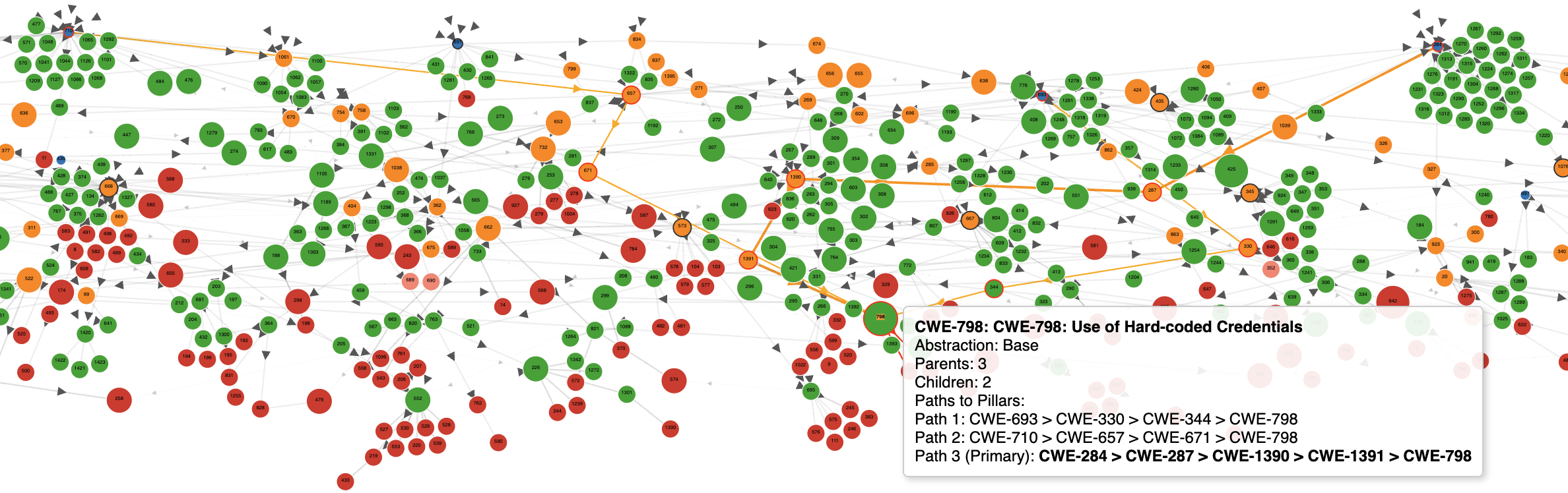
CWE-798 appears in 3 different chains. Only one path is the primary path.

Info

This raises the question of which chain(s) do we use

the shortest chain?
all the chains?
a selected chain?

For all chains: - the logic is the same always - the Recall and F1 will be lower if the CWE that appears in multiple chains is in the Predicted set

For CWEs with multiple parents, the “best” answer for mapping is the Primary parent and path*.

Each weakness can have one and only one ChildOf relationship that’s labeled “Primary” for each view.

Using all 3 chains for CWE-798:¶

Benchmark: CWE-912, CWE-798
Prediction: CWE-321, CWE-912

Chains used (excluding CWE-1000 Root):

CWE-912 Chain: CWE-710 > CWE-684 > CWE-912
CWE-798 Chains:
Chain 1: CWE-693 > CWE-330 > CWE-344 > CWE-798
Chain 2: CWE-710 > CWE-657 > CWE-671 > CWE-798
Chain 3 (Primary): CWE-284 > CWE-287 > CWE-1390 > CWE-1391 > CWE-798
CWE-321 Chain: CWE-284 > CWE-287 > CWE-1390 > CWE-1391 > CWE-798 > CWE-321

Augment sets:

Benchmark (Y):
CWE-912 ancestors: {CWE-710, CWE-684}
CWE-798 ancestors (all chains): {CWE-693, CWE-330, CWE-344, CWE-710, CWE-657, CWE-671, CWE-284, CWE-287, CWE-1390, CWE-1391}
Y_aug = {CWE-912, CWE-798, CWE-710, CWE-684, CWE-693, CWE-330, CWE-344, CWE-657, CWE-671, CWE-284, CWE-287, CWE-1390, CWE-1391}
|Y_aug| = 13
Prediction (Ŷ):
CWE-321 ancestors: {CWE-798, CWE-1391, CWE-1390, CWE-287, CWE-284}
CWE-912 ancestors: {CWE-710, CWE-684}
Ŷ_aug = {CWE-321, CWE-912, CWE-798, CWE-1391, CWE-1390, CWE-287, CWE-284, CWE-710, CWE-684}
|Ŷ_aug| = 9

Calculate metrics:

Intersection: {CWE-912, CWE-798, CWE-710, CWE-684, CWE-284, CWE-287, CWE-1390, CWE-1391} (|Intersection| = 8)
Precision (hP): $\frac{8}{9} \approx 0.889$
Recall (hR): $\frac{8}{13} \approx 0.615$
F-score (hF): $\frac{2 \times 0.889 \times 0.615}{0.889 + 0.615} \approx 0.727$

Result: Approx. 0.727, capturing key overlaps but diluted recall due to multiple ancestor paths.

Using only the Primary Path (Chain 3):¶

Benchmark: CWE-912, CWE-798
Prediction: CWE-321, CWE-912

Chains used:

CWE-912: CWE-710 > CWE-684 > CWE-912
CWE-798 Primary only: CWE-284 > CWE-287 > CWE-1390 > CWE-1391 > CWE-798
CWE-321: CWE-284 > CWE-287 > CWE-1390 > CWE-1391 > CWE-798 > CWE-321

Augment sets:

Benchmark (Y):
CWE-912 ancestors: {CWE-710, CWE-684}
CWE-798 ancestors (Primary path): {CWE-284, CWE-287, CWE-1390, CWE-1391}
Y_aug = {CWE-912, CWE-798, CWE-710, CWE-684, CWE-284, CWE-287, CWE-1390, CWE-1391}
|Y_aug| = 8
Prediction (Ŷ) (same as above): {CWE-321, CWE-912, CWE-798, CWE-1391, CWE-1390, CWE-287, CWE-284, CWE-710, CWE-684}
|Ŷ_aug| = 9

Calculate metrics:

Intersection (same as before): |Intersection| = 8
Precision (hP): $\frac{8}{9} \approx 0.889$
Recall (hR): $\frac{8}{8} = 1.0$
F-score (hF): $\frac{2 \times 0.889 \times 1.0}{0.889 + 1.0} \approx 0.941$

Result: Approx. 0.941, higher recall from narrower focus on primary path.

Using one non-primary path (Chain 1: CWE-693 > CWE-330 > CWE-344 > CWE-798):¶

Benchmark: CWE-912, CWE-798
Prediction: CWE-321, CWE-912

Chains used:

CWE-912: CWE-710 > CWE-684 > CWE-912
CWE-798 (Non-primary): CWE-693 > CWE-330 > CWE-344 > CWE-798
CWE-321: CWE-284 > CWE-287 > CWE-1390 > CWE-1391 > CWE-798 > CWE-321

Augment sets:

Benchmark (Y):
CWE-912 ancestors: {CWE-710, CWE-684}
CWE-798 ancestors (Chain 1): {CWE-693, CWE-330, CWE-344}
Y_aug = {CWE-912, CWE-798, CWE-710, CWE-684, CWE-693, CWE-330, CWE-344}
|Y_aug| = 7
Prediction (Ŷ) (same as above): |Ŷ_aug| = 9

Calculate metrics:

Intersection: {CWE-912, CWE-798, CWE-710, CWE-684} (|Intersection| = 4)
Precision (hP): $\frac{4}{9} \approx 0.444$
Recall (hR): $\frac{4}{7} \approx 0.571$
F-score (hF): $\frac{2 \times 0.444 \times 0.571}{0.444 + 0.571} \approx 0.500$

Result: Approx. 0.500, significantly lower, highlighting sensitivity to chosen paths.

Summary of Results¶

Scenario	Precision (hP)	Recall (hR)	F-score (hF)
All 3 Chains	0.889	0.615	0.727
Primary Path Only	0.889	1.000	0.941
Non-primary Path (Chain 1)	0.444	0.571	0.500

This clearly demonstrates how significantly path selection affects scoring. Using the primary path achieves the highest performance by aligning predictions with the benchmark’s primary hierarchical representation.

Example 8: "Similar CWEs" Prediction on a Different Branch¶

CWE-125: Out-of-bounds Read and CWE-476: NULL Pointer Dereference conceptually share high-level similarities (both being related to memory handling errors)

Paths to Pillars CWE-125: Out-of-bounds Read

Path 1 (Primary): CWE-664 > CWE-118 > CWE-119 > CWE-125

Paths to Pillars CWE-476: NULL Pointer Dereference

Path 1 (Primary): CWE-710 > CWE-476
Path 2: CWE-703 > CWE-754 > CWE-476

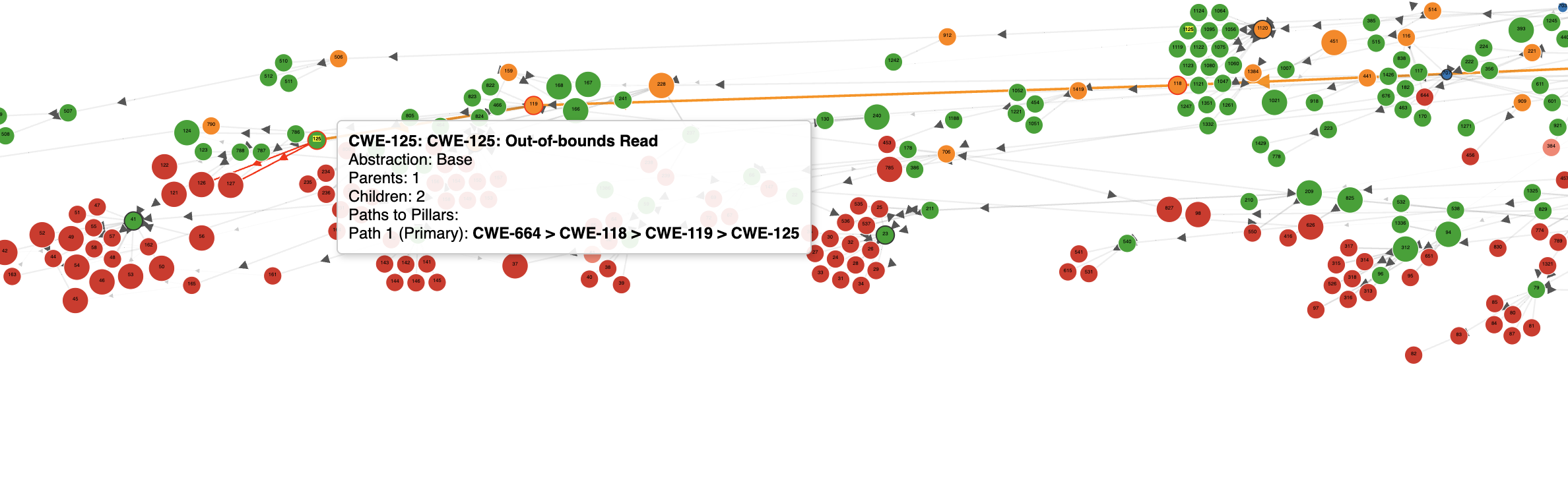
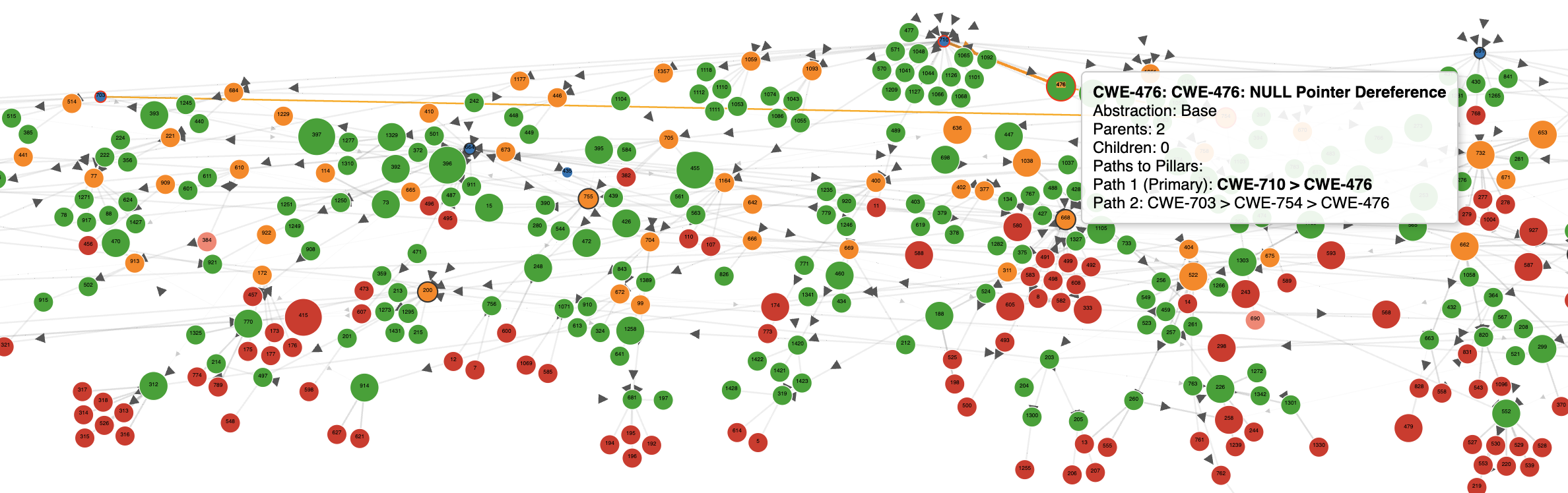
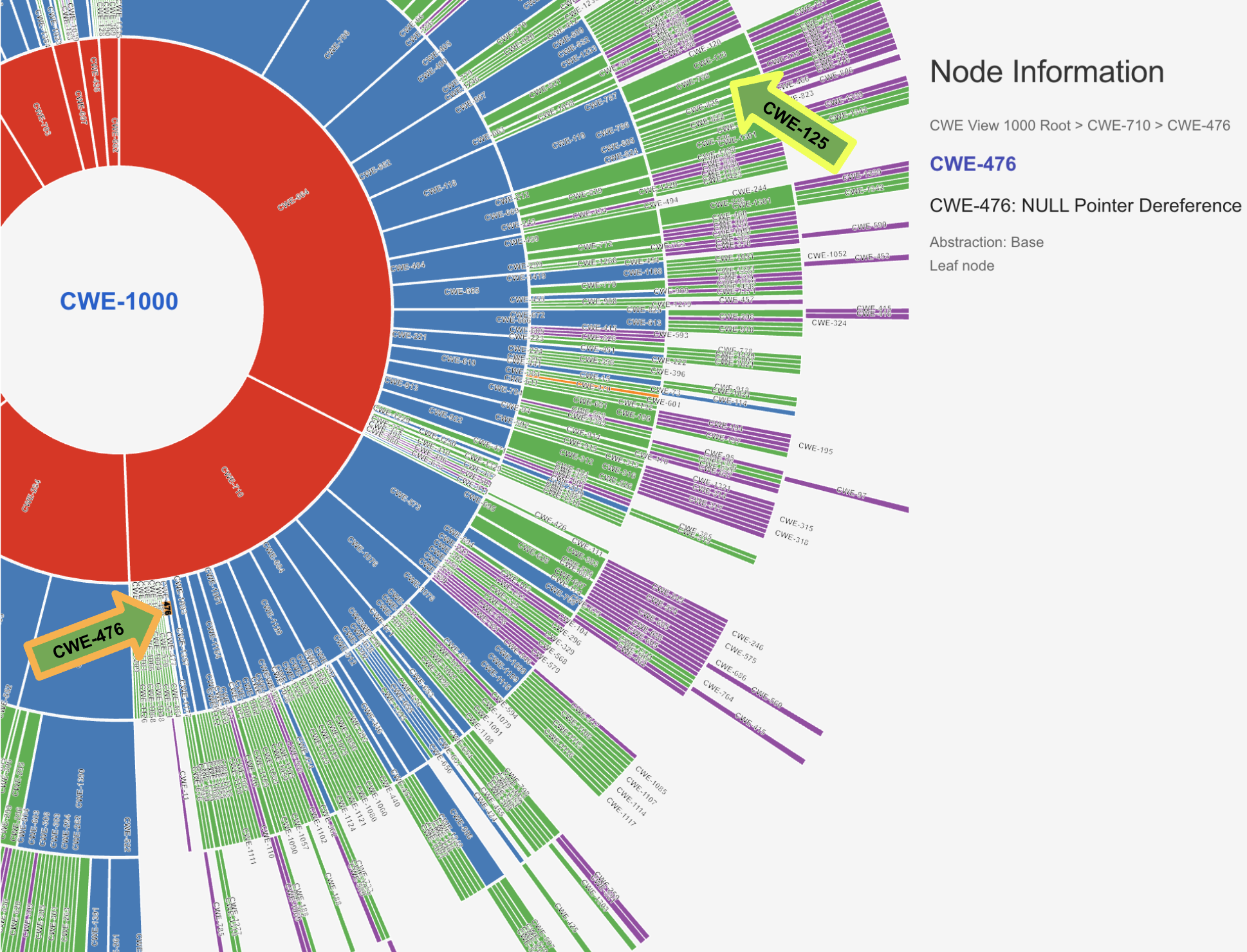
Calculate metrics:

Intersection: Empty set (no common ancestors between CWE-125 and CWE-476 paths)
Precision (hP): 0.0
Recall (hR): 0.0
F-score (hF): 0.0

Info

These two CWEs conceptually share high-level similarities (both being related to memory handling errors), but strict hierarchical scoring will not award any partial credit unless they explicitly share ancestors within the defined hierarchy.

5. Advantages of HCSS¶

Theoretical Grounding: Based on established research in hierarchical multi-label classification
Semantic Awareness: Incorporates the CWE hierarchy structure to reward closeness
Balanced Evaluation: Captures both precision and recall aspects
Interpretable: Produces normalized scores in a meaningful range
Flexibility: Supports both micro and macro averaging for different analysis needs
Standardized: Aligns with scientific evaluation practices for comparable results

6. Implementation Recommendations¶

Use the MITRE CWE XML data to build the hierarchy graph
Consider implementing optional weights for edges based on abstraction levels
Provide both micro and macro-averaged scores for comprehensive evaluation
Include standard metrics alongside HCSS for comparative context

This HCSS framework provides a robust, theoretically sound approach to evaluating automated CVE-to-CWE assignments, directly addressing the multi-label and hierarchical nature of the problem.

Ended: Scoring

CVE-CWE Dataset Schema and Example Layout¶

This document defines the JSON schema, example record, and directory structure used in the CVE-CWE Root Cause Mapping dataset. It serves as the "how" counterpart to the requirements document.

JSON Schema¶

{
  "$schema": "https://json-schema.org/draft/2020-12/schema",
  "title": "CVE_CWE_Record",
  "type": "object",
  "required": ["cve_id", "cwe_ids", "year", "description", "ref_links"],
  "properties": {
    "cve_id": {
      "type": "string",
      "pattern": "^CVE-\\d{4}-\\d{4,}$"
    },
    "cwe_ids": {
      "type": "array",
      "items": {
        "type": "string",
        "pattern": "^CWE-\\d+$"
      },
      "minItems": 1
    },
    "year": {
      "type": "integer",
      "minimum": 1999
    },
    "description": {
      "type": "string"
    },
    "ref_links": {
      "type": "array",
      "items": {
        "type": "string",
        "format": "uri"
      }
    },
    "ref_summaries": {
      "type": "array",
      "items": {
        "type": "string"
      },
      "default": []
    },
    "keyphrases": {
      "type": "array",
      "items": {
        "type": "string"
      },
      "default": []
    },
    "quality_flags": {
      "type": "array",
      "items": {
        "type": "string"
      },
      "default": []
    },
    "consensus_cna_score": {
      "type": "number",
      "minimum": 0,
      "maximum": 100
    },
    "consensus_desc_score": {
      "type": "number",
      "minimum": 0,
      "maximum": 100
    }
  }
}

Example Record¶

{
  "cve_id": "CVE-2024-29009",
  "cwe_ids": ["CWE-352"],
  "year": 2024,
  "description": "CWE-352 Cross-Site Request Forgery (CSRF)",
  "ref_links": [
    "https://nvd.nist.gov/vuln/detail/CVE-2024-29009"
  ],
  "ref_summaries": [
    "Summary of reference content goes here"
  ],
  "keyphrases": [
    "cross-site request forgery",
    "unauthenticated action"
  ],
  "quality_flags": [],
  "consensus_cna_score": 100,
  "consensus_desc_score": 92
}

Example Directory Layout¶

top_level/
├── full.jsonl              # All records, one per line (gold labels)
├── schema.json             # JSON Schema (Draft 2020‑12)
├── scripts/
│   ├── fetch.py            # Pull raw NVD entries
│   ├── clean.py            # Convert to schema format; deduplication, keyphrases
│   ├── benchmark.py        # Compare mapping predictions against benchmark
│   └── utils.py            # Shared helpers (e.g., semantic similarity)
├── README.md
├── LICENSE
├── Feedback.md
├── MaintenancePlan.md
└── validations/
    ├── schema_validator.py     # Validates schema compliance
    ├── requirements_check.py   # Verifies dataset meets core REQs
    └── stats_summary.py        # Reports on token lengths, distribution, etc.

Notes¶

Fields like keyphrases, quality_flags, and ref_summaries are optional but recommended.
consensus_*_score fields are optional but align with REQ_CONSENSUS_CNA_SCORE and REQ_CONSENSUS_DESC_SCORE.
All code and schema validation must use Draft 2020-12.

This structure supports both ease of use and future extensibility, including automation for quality validation and benchmarking.

Top25 Dataset ↵

Top25 2022, 2023 EDA¶

Overview

This section outlines the Top25 dataset.

See the CWE Top 25 Methodology for context on how the Top25 was created.

Introduction¶

The Top 25 dataset contains

9792 CVE-CWE mappings for 2023 dataset
9712 CVE-CWE mappings for 2022 dataset

where a mapping is one row with one CWE per CVE.

There may be multiple rows with the same CVE to reflect multiple CWEs mapped to that CVE.

Top25 Remap¶

Pre-Remap¶

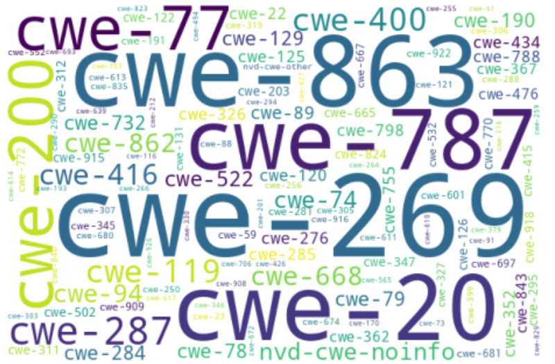
242 Unique CWE entries (including these that are not CWEs):

nvd-cwe-noinfo

Post-Remap¶

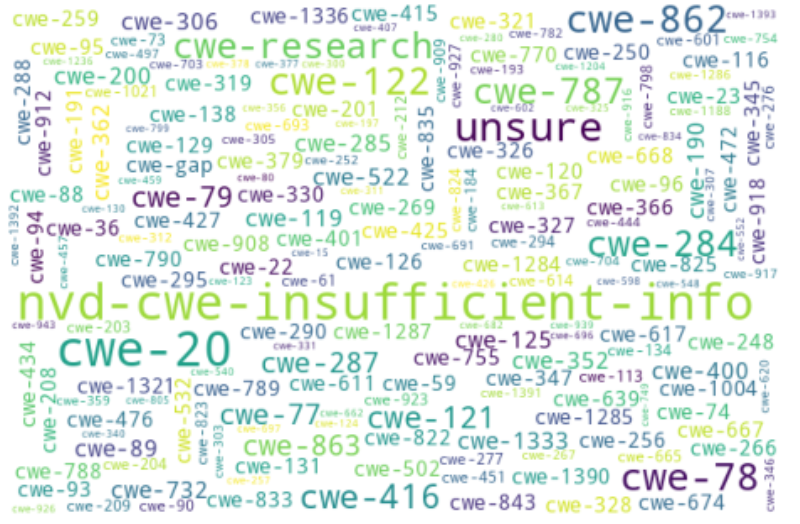
481 Unique CWE entries (including these that are not CWEs):

nvd-cwe-insufficient-info 7.4%
unsure 5.1%
cwe-research 3.1%

Observations

Comparing CWE word clouds, some things are clear

The Top 25 dataset contains double the number of unique CWEs compared to prior to remapping.
The mappings are more fine grained

The number of unique CWEs per CVE is approximately the same for 2022, 2023.

Counts of CWEs per CVE¶

Distribution of counts of CWEs per CVE after Top 25 remapping i.e. how many CVEs have 1 vs 2 vs 3... CWEs per (REQ_COVERAGE_MULTIPLE_CWES)?

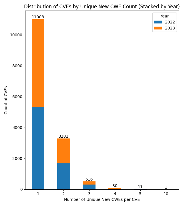
Observations

The number of unique CWEs per CVE is approximately the same for 2022, 2023.

Counts of CVEs per CWE¶

Distribution of counts of CVEs per CWEs i.e. how many CVE examples per CWE do we have per (REQ_COVERAGE_MIN_ENTRIES_PER_CWE)?

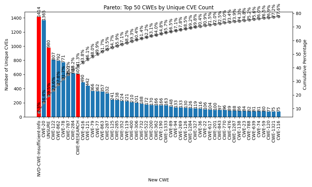
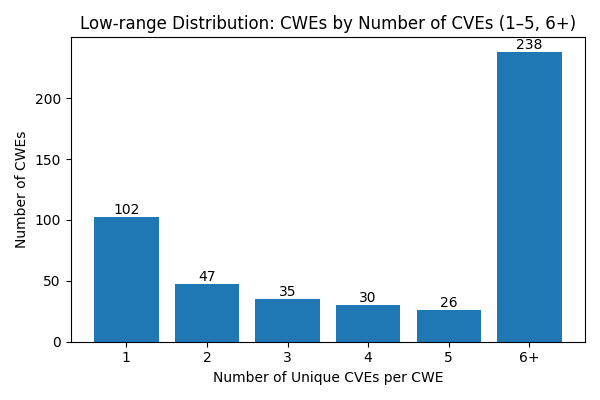
Distribution by Hierarchy¶

Tip

Interact with the sunburst showing counts of CVEs per CWE from the Top25 2022, 2023 data

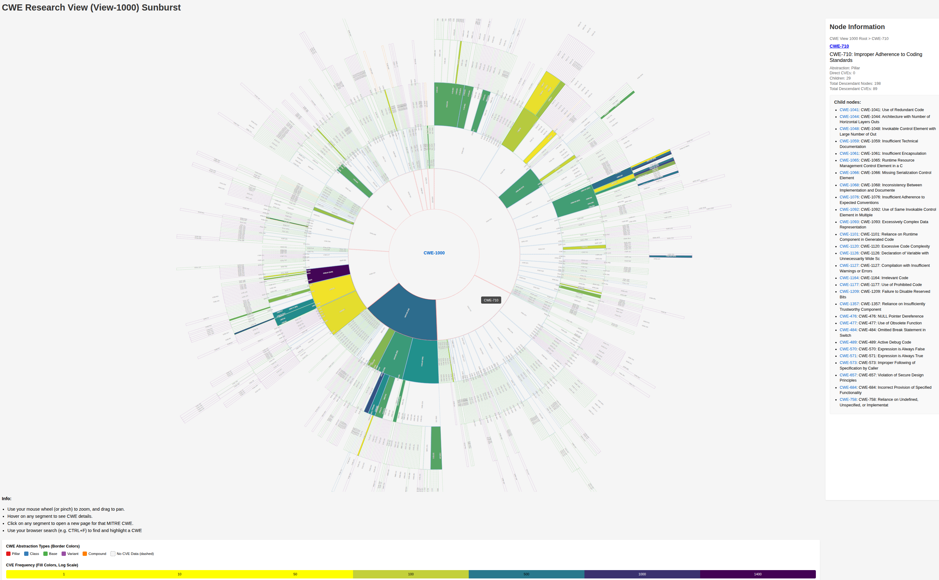interactive sunburst showing counts of CVEs per CWE from the Top25 2022, 2023 data

Observations

The Top 50 CWEs by count, account for 77.6% of all CVEs.

~210 CWEs of ~480 have less than 5 CVEs.

From the interactive sunburst showing counts of CVEs per CWE from the Top25 2022, 2023 data, we can see that

some CWE Pillars have very few CVEs assigned e.g.

CWE-435: Improper Interaction Between Multiple Correctly-Behaving Entities and CWE-697: Incorrect Comparison have a total of 0 CVEs in descendant CWEs.
CWE-710: Improper Adherence to Coding Standards has a total of 89 CVEs in descendant CWEs.

The CWE Pillars with most CVEs assigned are

Component	Symbol / Notation	Definition / Calculation	Notes
Inputs (per CVE i)
True CWE Set	\(Y_i\)	Set of ground truth CWE IDs for CVE i.	e.g.,
Predicted CWE Set	\(\hat{Y}_i\)	Set of predicted CWE IDs for CVE i.	e.g.,
CWE Hierarchy	\(H\)	Data structure representing CWE nodes and relationships (ParentOf/ChildOf).	Parsed from MITRE XML data.
Core Functions
Ancestor Set	\(Ancestors(c, H)\)	Set of all ancestor CWE IDs of node c in hierarchy H.	Includes transitive ancestors up to the root(s).
Augmented Set	\(Y_{aug,i}, \hat{Y}_{aug,i}\)	\(Y_{aug,i} = Y_i \cup \bigcup_{y \in Y_i} Ancestors(y, H)\) \(\hat{Y}_{aug,i} = \hat{Y}_i \cup \bigcup_{\hat{y} \in \hat{Y}_i} Ancestors(\hat{y}, H)\)	Includes original nodes plus all their ancestors.
Per-CVE Metrics		Calculated for each CVE \(i=1...N\).
Intersection Size	\(Intersection_i\)	$	\hat{Y}{aug,i} \cap Y
Hierarchical Precision	\(hP_i\)	\(\frac{Intersection_i}{\hat{Y}_{aug,i}}\) (handle division by zero)	Proportion of augmented predictions that are in the augmented true set.
Hierarchical Recall	\(hR_i\)	\(\frac{Intersection_i}{Y_{aug,i}}\) (handle division by zero)	Proportion of augmented true labels that are in the augmented predicted set.
Hierarchical F-measure	\(hF_i\)	\(\frac{2 \times hP_i \times hR_i}{hP_i + hR_i}\) (handle division by zero)	Harmonic mean of \(hP_i\) and \(hR_i\).
Aggregated Metrics		Calculated over the entire dataset of N CVEs.
Macro-hP	\(hP_{macro}\)	\(\frac{1}{N} \sum_{i=1}^{N}hP_i\)	Average per-CVE hierarchical precision.
Macro-hR	\(hR_{macro}\)	\(\frac{1}{N} \sum_{i=1}^{N} hR_i\)	Average per-CVE hierarchical recall.
Macro-hF	\(hF_{macro}\)	\(\frac{2 \times hP_{macro} \times hR_{macro}}{hP_{macro} + hR_{macro}}\) (handle division by zero)	Overall F-measure based on macro-averaged P & R.
Micro-hP	\(hP_{micro}\)	\(\frac{\sum_{i=1}^{N} Intersection_i}{\sum_{i=1}^{N}}\)	\({\hat{Y}_{aug,i}}\) (handle division by zero)
Micro-hR	\(hR_{micro}\)	\(\frac{\sum_{i=1}^{N} Intersection_i}{\sum_{i=1}^{N}}\)	\({Y_{aug,i}}\) (handle division by zero)
Micro-hF	\(hF_{micro}\)	\(\frac{2 \times hP_{micro} \times hR_{micro}}{hP_{micro} + hR_{micro}}\) (handle division by zero)	Overall F-measure based on micro-averaged P & R.
Optional Diagnostic
Closeness Function	\(sim(c_1, c_2)\)	e.g., \(sim_{WP}(c_1, c_2) = \frac{2 \times depth(LCS(c_1, c_2))}{depth(c_1) + depth(c_2)}\)	Quantifies similarity (0-1) between two CWE nodes. Used for analysis.